在R中拟合正态分布

Question

我正在使用以下代码来拟合正态分布。 "b" 的数据集链接（太大无法直接发布）为：

b 的链接

setwd("xxxxxx")
library(fitdistrplus)

require(MASS)
tazur <-read.csv("b", header= TRUE, sep=",")
claims<-tazur$b
a<-log(claims)
plot(hist(a))

绘制直方图后，似乎正态分布适合拟合数据。

f1n <- fitdistr(claims,"normal")
summary(f1n)

#Length Class  Mode   
#estimate 2      -none- numeric
#sd       2      -none- numeric
#vcov     4      -none- numeric
#n        1      -none- numeric
#loglik   1      -none- numeric

plot(f1n)

但是当我尝试绘制拟合的分布时，我得到了

Error in xy.coords(x, y, xlabel, ylabel, log) : 

  'x' is a list, but does not have components 'x' and 'y'

甚至f1n的摘要统计数据也不准确。有什么想法吗？

- zkhan

---

m <- mean(claims); s <- sd(claims) - Hong Ooi

Answer 1

看起来你在MASS::fitdistr和fitdistrplus::fitdist之间产生了混淆。

• MASS::fitdistr返回“fitdistr”类的对象，该类没有绘图方法。因此，您需要提取估计参数并自己绘制估计密度曲线。
• 我不知道为什么要加载fitdistrplus包，因为您的函数调用明确显示您正在使用MASS。无论如何，fitdistrplus有一个名为fitdist的函数，该函数返回“fitdist”类的对象。这个类有绘图方法，但对于由MASS返回的“fitdistr”不起作用。

我将向您展示如何使用这两个包。

## reproducible example
set.seed(0); x <- rnorm(500)

---

使用 MASS::fitdistr 函数

由于没有可用的绘图方法，我们需要自己完成。

library(MASS)
fit <- fitdistr(x, "normal")
class(fit)
# [1] "fitdistr"

para <- fit$estimate
#         mean            sd 
#-0.0002000485  0.9886248515 

hist(x, prob = TRUE)
curve(dnorm(x, para[1], para[2]), col = 2, add = TRUE)

---

使用 fitdistrplus::fitdist

library(fitdistrplus)
FIT <- fitdist(x, "norm")    ## note: it is "norm" not "normal"
class(FIT)
# [1] "fitdist"

plot(FIT)    ## use method `plot.fitdist`

- Zheyuan Li

---

你觉得值得说一下，通过mean(x)、sd(x)等方法来最优地估计正态分布的参数吗？ - Ben Bolker

是的（虽然平均数的不确定性在封闭形式中也很容易 - 标准差的不确定性有点麻烦） - Ben Bolker

如果是Wald标准误差，那么我认为Delta方法应该适用：SE(f(x))约等于df/dx * SE(x) ... 在这种情况下，f(x)是sqrt(x)，所以如果我算对了的话，SE(sd) = 0.5/sqrt(x)*SE(var)。(如果您有基于似然比检验的区间，则它们在变换下不变，因此只需取区间端点的平方根即可。) - Ben Bolker

Answer 2

上一个答案的回顾

在之前的答案中，我没有提到两种方法之间的区别。通常情况下，如果我们选择最大似然推断，我建议使用MASS::fitdistr，因为对于许多基本分布，它执行精确推断而不是数值优化。 ?fitdistr文档已经很清楚了：

对于正态，对数正态，几何，指数和泊松分布，使用闭合形式的MLE（和精确标准误差），不应提供“start”。

对于所有其他分布，使用直接优化对数似然来计算观察到的信息矩阵的估计标准误差，通过数值近似计算。 对于一维问题，使用Nelder-Mead方法，对于多维问题，使用BFGS方法，除非提供了名为“lower”或“upper”的参数（在使用“L-BFGS-B”时）或显式提供了“method”。

另一方面，fitdistrplus::fitdist始终以数字方式进行推断，即使存在精确推断也是如此。 当然，fitdist的优点在于更多的推断原则可用：

通过最大似然（mle），矩匹配（mme），分位数匹配（qme）或最大化拟合度评估（mge）将单变量分布适合非截断数据。

---

此答案的目的

本答案将探讨正态分布的精确推断。它将具有理论味道，但没有似然原则的证明；仅给出结果。基于这些结果，我们编写自己的R函数进行精确推断，可以与MASS::fitdistr进行比较。另一方面，为了与fitdistrplus :: fitdist进行比较，我们使用optim以数字方式最小化负对数似然函数。

这是一个学习统计和相对高级使用optim的绝佳机会。为方便起见，我将估计尺度参数：方差，而不是标准误差。

---

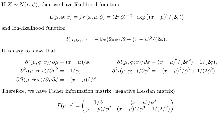
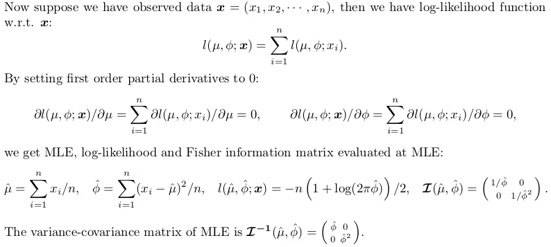
正态分布的精确推断

---

自己编写推断函数

以下代码已经很好地注释了。有一个开关exact。如果设置为FALSE，则选择数字解决方案。

## fitting a normal distribution
fitnormal <- function (x, exact = TRUE) {
  if (exact) {
    ################################################
    ## Exact inference based on likelihood theory ##
    ################################################
    ## minimum negative log-likelihood (maximum log-likelihood) estimator of `mu` and `phi = sigma ^ 2`
    n <- length(x)
    mu <- sum(x) / n
    phi <- crossprod(x - mu)[1L] / n  # (a bised estimator, though)
    ## inverse of Fisher information matrix evaluated at MLE
    invI <- matrix(c(phi, 0, 0, phi * phi), 2L,
                   dimnames = list(c("mu", "sigma2"), c("mu", "sigma2")))
    ## log-likelihood at MLE
    loglik <- -(n / 2) * (log(2 * pi * phi) + 1)
    ## return
    return(list(theta = c(mu = mu, sigma2 = phi), vcov = invI, loglik = loglik, n = n))
    }
  else {
    ##################################################################
    ## Numerical optimization by minimizing negative log-likelihood ##
    ##################################################################
    ## negative log-likelihood function
    ## define `theta = c(mu, phi)` in order to use `optim`
    nllik <- function (theta, x) {
      (length(x) / 2) * log(2 * pi * theta[2]) + crossprod(x - theta[1])[1] / (2 * theta[2])
      }
    ## gradient function (remember to flip the sign when using partial derivative result of log-likelihood)
    ## define `theta = c(mu, phi)` in order to use `optim`
    gradient <- function (theta, x) {
      pl2pmu <- -sum(x - theta[1]) / theta[2]
      pl2pphi <- -crossprod(x - theta[1])[1] / (2 * theta[2] ^ 2) + length(x) / (2 * theta[2])
      c(pl2pmu, pl2pphi)
      }
    ## ask `optim` to return Hessian matrix by `hessian = TRUE`
    ## use "..." part to pass `x` as additional / further argument to "fn" and "gn"
    ## note, we want `phi` as positive so box constraint is used, with "L-BFGS-B" method chosen
    init <- c(sample(x, 1), sample(abs(x) + 0.1, 1))  ## arbitrary valid starting values
    z <- optim(par = init, fn = nllik, gr = gradient, x = x, lower = c(-Inf, 0), method = "L-BFGS-B", hessian = TRUE)
    ## post processing ##
    theta <- z$par
    loglik <- -z$value  ## flip the sign to get log-likelihood
    n <- length(x)
    ## Fisher information matrix (don't flip the sign as this is the Hessian for negative log-likelihood)
    I <- z$hessian / n  ## remember to take average to get mean
    invI <- solve(I, diag(2L))  ## numerical inverse
    dimnames(invI) <- list(c("mu", "sigma2"), c("mu", "sigma2"))
    ## return
    return(list(theta = theta, vcov = invI, loglik = loglik, n = n))
    }
  }

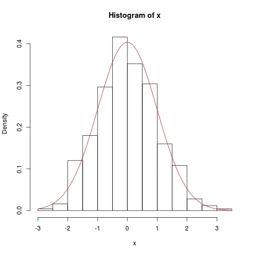
我们仍然使用之前的数据进行测试：

set.seed(0); x <- rnorm(500)

## exact inference
fit <- fitnormal(x)

#$theta
#           mu        sigma2 
#-0.0002000485  0.9773790969 
#
#$vcov
#              mu    sigma2
#mu     0.9773791 0.0000000
#sigma2 0.0000000 0.9552699
#
#$loglik
#[1] -703.7491
#
#$n
#[1] 500

hist(x, prob = TRUE)
curve(dnorm(x, fit$theta[1], sqrt(fit$theta[2])), add = TRUE, col = 2)

数值方法也相当准确，只是方差协方差矩阵的对角线上并非完全为0：

fitnormal(x, FALSE)

#$theta
#[1] -0.0002235315  0.9773732277
#
#$vcov
#                 mu       sigma2
#mu     9.773826e-01 5.359978e-06
#sigma2 5.359978e-06 1.910561e+00
#
#$loglik
#[1] -703.7491
#
#$n
#[1] 500

- Zheyuan Li

---

让我开心的是，在Stack Overflow上找到了M估计理论，向你致敬。 - Abbraxas