以下代码是一般答案的版本,但经过修正和澄清。
import numpy as np
import pandas as pd
import scipy.stats as st
import statsmodels.api as sm
import matplotlib as mpl
import matplotlib.pyplot as plt
import math
import random
mpl.style.use("ggplot")
def danoes_formula(data):
"""
DANOE'S FORMULA
https://en.wikipedia.org/wiki/Histogram#Doane's_formula
"""
N = len(data)
skewness = st.skew(data)
sigma_g1 = math.sqrt((6*(N-2))/((N+1)*(N+3)))
num_bins = 1 + math.log(N,2) + math.log(1+abs(skewness)/sigma_g1,2)
num_bins = round(num_bins)
return num_bins
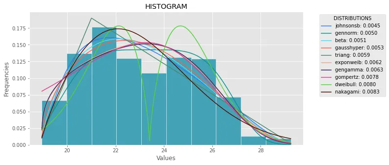
def plot_histogram(data, results, n):
N_DISTRIBUTIONS = {k: results[k] for k in list(results)[:n]}
plt.figure(figsize=(10, 5))
plt.hist(data, density=True, ec='white', color=(63/235, 149/235, 170/235))
plt.title('HISTOGRAM')
plt.xlabel('Values')
plt.ylabel('Frequencies')
for distribution, result in N_DISTRIBUTIONS.items():
sse = result[0]
arg = result[1]
loc = result[2]
scale = result[3]
x_plot = np.linspace(min(data), max(data), 1000)
y_plot = distribution.pdf(x_plot, loc=loc, scale=scale, *arg)
plt.plot(x_plot, y_plot, label=str(distribution)[32:-34] + ": " + str(sse)[0:6], color=(random.uniform(0, 1), random.uniform(0, 1), random.uniform(0, 1)))
plt.legend(title='DISTRIBUTIONS', bbox_to_anchor=(1.05, 1), loc='upper left')
plt.show()
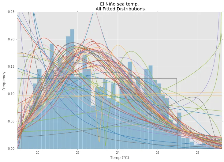
def fit_data(data):
ALL_DISTRIBUTIONS = [
st.alpha,st.anglit,st.arcsine,st.beta,st.betaprime,st.bradford,st.burr,st.cauchy,st.chi,st.chi2,st.cosine,
st.dgamma,st.dweibull,st.erlang,st.expon,st.exponnorm,st.exponweib,st.exponpow,st.f,st.fatiguelife,st.fisk,
st.foldcauchy,st.foldnorm, st.genlogistic,st.genpareto,st.gennorm,st.genexpon,
st.genextreme,st.gausshyper,st.gamma,st.gengamma,st.genhalflogistic,st.gilbrat,st.gompertz,st.gumbel_r,
st.gumbel_l,st.halfcauchy,st.halflogistic,st.halfnorm,st.halfgennorm,st.hypsecant,st.invgamma,st.invgauss,
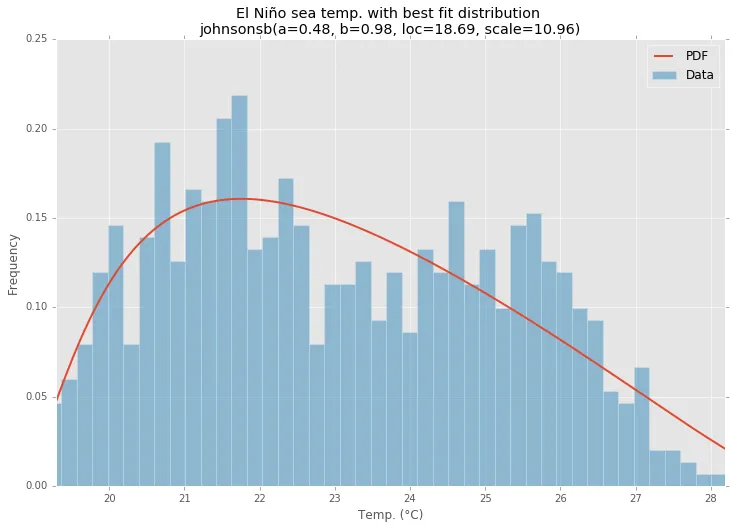
st.invweibull,st.johnsonsb,st.johnsonsu,st.ksone,st.kstwobign,st.laplace,st.levy,st.levy_l,
st.logistic,st.loggamma,st.loglaplace,st.lognorm,st.lomax,st.maxwell,st.mielke,st.nakagami,st.ncx2,st.ncf,
st.nct,st.norm,st.pareto,st.pearson3,st.powerlaw,st.powerlognorm,st.powernorm,st.rdist,st.reciprocal,
st.rayleigh,st.rice,st.recipinvgauss,st.semicircular,st.t,st.triang,st.truncexpon,st.truncnorm,st.tukeylambda,
st.uniform,st.vonmises,st.vonmises_line,st.wald,st.weibull_min,st.weibull_max,st.wrapcauchy
]
MY_DISTRIBUTIONS = [st.beta, st.expon, st.norm, st.uniform, st.johnsonsb, st.gennorm, st.gausshyper]
num_bins = danoes_formula(data)
frequencies, bin_edges = np.histogram(data, num_bins, density=True)
central_values = [(bin_edges[i] + bin_edges[i+1])/2 for i in range(len(bin_edges)-1)]
results = {}
for distribution in MY_DISTRIBUTIONS:
params = distribution.fit(data)
arg = params[:-2]
loc = params[-2]
scale = params[-1]
pdf_values = [distribution.pdf(c, loc=loc, scale=scale, *arg) for c in central_values]
sse = np.sum(np.power(frequencies - pdf_values, 2.0))
results[distribution] = [sse, arg, loc, scale]
results = {k: results[k] for k in sorted(results, key=results.get)}
return results
def main():
data = pd.Series(sm.datasets.elnino.load_pandas().data.set_index('YEAR').values.ravel())
results = fit_data(data)
plot_histogram(data, results, 5)
if __name__ == "__main__":
main()