如何在Python中从正态概率密度函数中寻找概率？

Question

基本上，我使用平均值和标准差的值绘制了一个正态曲线。y轴给出了概率密度。

如何在x轴上的某个特定值“x”处找到概率？是否有Python函数可以实现或者该如何编写代码？

- Prakrut Chauhan

---

如果您有一个连续分布，根据定义，任何值的概率都是零...您唯一能问的问题是x在某个值之上/之下或在某个范围内的概率是多少。然后这应该回答https://www.dummies.com/education/math/statistics/how-to-find-statistical-probabilities-in-a-normal-distribution/ 或者我错过了什么？ - My Work

Answer 1

我不太确定你是否指的是概率密度函数，它是：

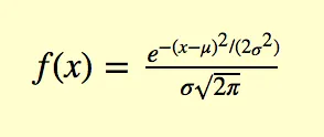
在给定均值和标准差的情况下。在Python中，您可以使用stats.norm.fit来获取概率，例如，我们有一些数据，其中拟合了正态分布：

from scipy import stats
import seaborn as sns
import numpy as np
import matplotlib.pyplot as plt

data = stats.norm.rvs(10,2,1000)

x = np.linspace(min(data),max(data),1000)
mu, var = stats.norm.fit(data)
p = stats.norm.pdf(x, mu, std)

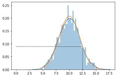
现在我们已经估算出了均值和标准差，我们使用概率密度函数来估算例如12.5的概率：

xval = 12.5
p_at_x = stats.norm.pdf(xval,mu,std)

我们可以绘制图表来查看它是否符合你的要求：

fig, ax = plt.subplots(1,1)
sns.distplot(data,bins=50,ax=ax)
plt.plot(x,p)
ax.hlines(p_at_x,0,xval,linestyle ="dotted")
ax.vlines(xval,0,p_at_x,linestyle ="dotted")

- StupidWolf

Answer 2

一个scipy.stat分布包括以下三种方法： pdf(x)：在x处的概率密度函数值。这是你所要求的。

cdf(x)：在x处的累积概率。 ppf(p)：cdf()的反函数。给出累积概率p的临界值。

import scipy.stats as stats
import matplotlib.pyplot as plt
import numpy as np
import pandas as pd
# plot a normal distribution and use scipy.stats to obtain
# probabilities and critical values (percentiles).
# Using scipy.stats, this can be done for any distribution
# listed in the documentation: https://docs.scipy.org/doc/scipy/reference/stats.html.
# scipy is included in the standard Anaconda python distribution.

loc = 0        # the mean
scale = 1      # the standard deviation
# a scipy.stats normal distribution
# scipy.stats supports 50+ continuous distributions.
d = stats.norm(loc, scale)

# a scipy.stat distribution includes these 3 methods:
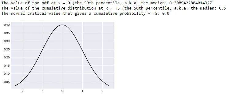
#   norm.pdf(x)     # the value of the pdf at x. This is what you asked for.
#   norm.cdf(x)     # the cumulative probability at x.
#   norm.ppf(p)     # the inverse of the cdf(). The critical value that gives cumulative probability, p.

# d.pdf(x) gives the probability you asked for.
print(f'The value of the pdf at x = 0 (the 50th percentile, a.k.a. the median: {d.pdf(0)}')
# d.cdf(x) gives the cumulative probability at x (x is a critical value of the normal distribution.
print(f'The value of the cumulative distribution at x = .5 (the 50th percentile, a.k.a. the median: {d.cdf(d.ppf(.5))}')
# d.ppf(p) is the inverse of cdf. The critical value that gives cumulative probability, p.
print(f'The normal critical value that gives a cumulative probability = .5: {d.ppf(.5)}')

# plot the distribution over these percentiles.
quantile_range = (.01, .99)
# generate sample_size quantile values for the x-axis
# of the plot of the probability distribution function (pdf)
sample_size = 100
x = np.linspace(d.ppf(quantile_range[0]), d.ppf(quantile_range[1]), sample_size)

y = d.pdf(x)        # return an array of probabilities (pdf values) for x
# setup the plot area
plt.style.use('seaborn-darkgrid')
fig, ax = plt.subplots()
# If ypu move your mouse along the curve, you will
# see the value of the pdf in in the lower left of the plot (mouse tips)
ax.plot(x, y, color='black', linewidth=1.5)

plt.show()
plt.close()

- tmck