我想对一些数据点拟合一个平面并绘制它。我目前的代码是:
import numpy as np
from mpl_toolkits.mplot3d import Axes3D
import matplotlib.pyplot as plt

points = [(1.1,2.1,8.1),
          (3.2,4.2,8.0),
          (5.3,1.3,8.2),
          (3.4,2.4,8.3),
          (1.5,4.5,8.0)]

xs, ys, zs = zip(*points)

fig = plt.figure()
ax = fig.add_subplot(111, projection='3d')

ax.scatter(xs, ys, zs)

point  = np.array([0.0, 0.0, 8.1])
normal = np.array([0.0, 0.0, 1.0])
d = -point.dot(normal)
xx, yy = np.meshgrid([-5,10], [-5,10])
z = (-normal[0] * xx - normal[1] * yy - d) * 1. /normal[2]
ax.plot_surface(xx, yy, z, alpha=0.2, color=[0,1,0])

ax.set_xlim(-10,10)
ax.set_ylim(-10,10)
ax.set_zlim(  0,10)

plt.show()
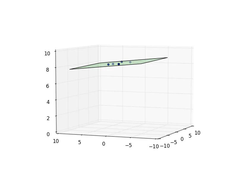
结果如下所示: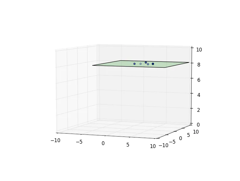
从目前的情况可以看出,我是手动创建这个平面的。如何计算它?我猜可能可以通过scipy.optimize.minimize实现。对于我来说,误差函数的类型并不那么重要。我认为最小二乘法(垂直点-平面距离)应该就可以了。如果有人能向我展示如何实现,那就太棒了。