在Python中计算累积分布函数（CDF）

Question

我该如何在Python中计算累积分布函数（CDF）？

我想从我有的点数组（离散分布）计算它，而不是使用连续分布，比如scipy中有的。

- wizbcn

---

使用 numpy.cumsum 怎么样？ - mdml

使用 numpy.cumsum，我认为您首先需要计算PDF，这是一种开销。 - wizbcn

你正在寻找经验分布函数（ECDF）。@DrV为您提供了一个简单版本。它也可以在statsmodels中找到。 - jlandercy

Answer 1

（如果我对问题的解释不正确，请谅解。如果问题是如何将离散概率密度函数转换为离散累积分布函数，那么如果样本等间距，则通过np.cumsum除以适当的常数即可。如果数组不等间距，则np.cumsum乘以点之间的距离即可。）

如果您有一个离散的样本数组，并且想知道样本的累积分布函数（CDF），则只需对数组进行排序即可。如果您查看排序后的结果，您会发现最小值表示0％，最大值表示100％。如果您想了解分布的50％值，只需查看排序后的数组元素，该元素位于排序后的数组中间。

让我们通过一个简单的例子来更深入地了解这个过程：

import matplotlib.pyplot as plt
import numpy as np

# create some randomly ddistributed data:
data = np.random.randn(10000)

# sort the data:
data_sorted = np.sort(data)

# calculate the proportional values of samples
p = 1. * np.arange(len(data)) / (len(data) - 1)

# plot the sorted data:
fig = plt.figure()
ax1 = fig.add_subplot(121)
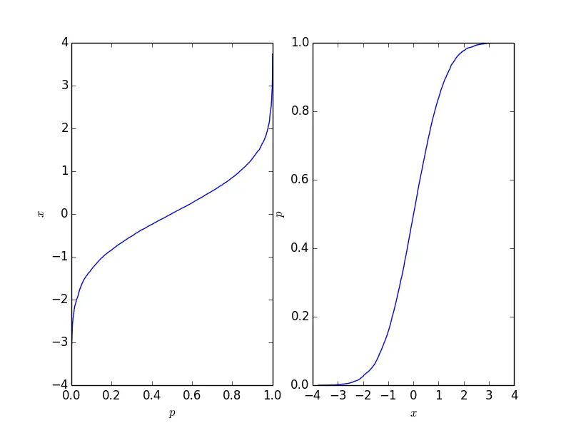
ax1.plot(p, data_sorted)
ax1.set_xlabel('$p$')
ax1.set_ylabel('$x$')

ax2 = fig.add_subplot(122)
ax2.plot(data_sorted, p)
ax2.set_xlabel('$x$')
ax2.set_ylabel('$p$')

这会生成以下图形，其中右侧的图形是传统的累积分布函数。它应该反映出点背后的过程的CDF，但自然地，只要点的数量有限，它就不会像那么长。

这个函数很容易反转，而它所需的形式取决于您的应用程序。

- DrV

---

太好了！谢谢你的回答。我不知道是否应该为此创建一个新问题，但是，如果我的数据有N个维度怎么办？（举个例子，假设有2个） - wizbcn

我可以翻译。您想知道如何获取可用的函数，但是对方提供的答案仅包含绘图。 - Tjorriemorrie

这个 np.linspace(0, 1, len(data)) 比 1. * arange(len(data)) / (len(data) - 1) 更加简洁。 - charmoniumQ

为了将其变成实际功能，您可以使用内插法进行翻译: f = lambda x: np.interp(x, p, data_sorted)。接下来，例如，您可以使用 f(0.5) 来获取中位数，但不要改变原来的意思。 - charmoniumQ

@charmoniumQ：我也喜欢使用 linspace，但值得一提的是最好使用 np.linspace(0, 1, len(data), endpoint=False) 或者 np.arange(len(data)) / len(data)，否则它不是CDF的无偏估计。我喜欢这篇帖子，其中有详细的解释：https://dev59.com/LXA75IYBdhLWcg3wlqSh#11692365。 - Nerxis

Answer 2

假设您知道数据的分布方式（即您了解数据的概率密度函数），那么在计算累积分布函数时，scipy 支持离散数据。

import numpy as np
import scipy
import matplotlib.pyplot as plt
import seaborn as sns

x = np.random.randn(10000) # generate samples from normal distribution (discrete data)
norm_cdf = scipy.stats.norm.cdf(x) # calculate the cdf - also discrete

# plot the cdf
sns.lineplot(x=x, y=norm_cdf)
plt.show()

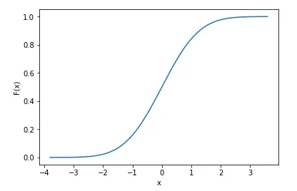
我们甚至可以打印累积分布函数的前几个值来展示它们是离散的。

print(norm_cdf[:10])
>>> array([0.39216484, 0.09554546, 0.71268696, 0.5007396 , 0.76484329,
       0.37920836, 0.86010018, 0.9191937 , 0.46374527, 0.4576634 ])

同样的方法用于计算多维cdf也是可行的：下面我们使用2d数据来说明。

mu = np.zeros(2) # mean vector
cov = np.array([[1,0.6],[0.6,1]]) # covariance matrix
# generate 2d normally distributed samples using 0 mean and the covariance matrix above
x = np.random.multivariate_normal(mean=mu, cov=cov, size=1000) # 1000 samples
norm_cdf = scipy.stats.norm.cdf(x)
print(norm_cdf.shape)
>>> (1000, 2)

在上面的例子中，我已经知道我的数据服从正态分布，这就是我使用 scipy.stats.norm() 的原因 - scipy 支持多种分布。但是，你需要事先了解你的数据如何分布，才能使用这样的函数。如果你不知道数据如何分布，并且只是使用任何分布来计算 cdf，那么你很可能会得到不正确的结果。

- PyRsquared

---

我不理解从正态分布中采样向量 x 的意义。相反，向量 x 应该是通过 linespace 函数来绘制你从 scipy.stats 中使用的参数化版本的 cdf。无论如何，OP要求非参数化的 CDF，他正在寻求离散但很可能意味着非参数化的 ECDF。 - jlandercy

Answer 3

经验累积分布函数是一个在数据集中准确跳跃的CDF。它是一个离散分布的CDF，该分布在每个值处放置质量，其中质量与值的频率成比例。由于质量之和必须为1，这些约束条件确定了经验CDF中每个跳跃的位置和高度。 给定一个值数组a，您可以通过先获取值的频率来计算经验CDF。numpy函数unique()在此非常有用，因为它不仅返回频率，还返回按排序顺序排列的值。要计算累积分布，请使用cumsum()函数并除以总和。以下函数返回排序后的值和相应的累积分布：

import numpy as np

def ecdf(a):
    x, counts = np.unique(a, return_counts=True)
    cusum = np.cumsum(counts)
    return x, cusum / cusum[-1]

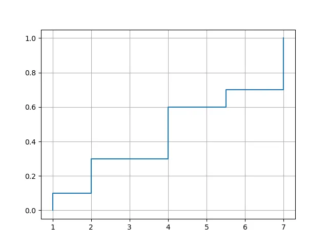
要绘制经验分布函数，您可以使用matplotlib的plot()函数。选项drawstyle='steps-post'确保跳跃发生在正确的位置。但是，您需要在最小数据值处强制进行跳跃，因此需要在x和y前面插入一个额外的元素。

import matplotlib.pyplot as plt

def plot_ecdf(a):
    x, y = ecdf(a)
    x = np.insert(x, 0, x[0])
    y = np.insert(y, 0, 0.)
    plt.plot(x, y, drawstyle='steps-post')
    plt.grid(True)
    plt.savefig('ecdf.png')

使用示例：

xvec = np.array([7,1,2,2,7,4,4,4,5.5,7])
plot_ecdf(xvec)

df = pd.DataFrame({'x':[7,1,2,2,7,4,4,4,5.5,7]})
plot_ecdf(df['x'])

带有输出结果：

- grand_chat

Answer 4

计算离散数列的CDF：

import numpy as np
pdf, bin_edges = np.histogram(
   data,        # array of data
   bins=500,    # specify the number of bins for distribution function
   density=True # True to return probability density function (pdf) instead of count
   )

cdf = np.cumsum(pdf*np.diff(bins_edges))

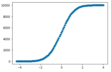
请注意，返回的数组pdf的长度为bins（这里是500），而bin_edges的长度为bins+1（这里是501）。

因此，要计算CDF即概率密度函数曲线下面积，我们可以使用Numpy的cumsum函数，简单地计算累积宽度(np.diff(bins_edges))乘以pdf 。

- Babak

---

我认为在代码的最后一行，你想用 bin_edges 而不是 bins_count，因此代码应该是：cdf = np.cumsum(pdf*np.diff(bin_edges))。 - Jim

Answer 5

这里提供了一种 pandas 的替代方案来计算经验 CDF，首先使用 pd.cut 将数据按照等距离的区间进行排序，然后使用 cumsum 计算分布。

def empirical_cdf(s: pd.Series, n_bins: int = 100):
    # Sort the data into `n_bins` evenly spaced bins:
    discretized = pd.cut(s, n_bins)
    # Count the number of datapoints in each bin:
    bin_counts = discretized.value_counts().sort_index().reset_index()
    # Calculate the locations of each bin as just the mean of the bin start and end:
    bin_counts["loc"] = (pd.IntervalIndex(bin_counts["index"]).left + pd.IntervalIndex(bin_counts["index"]).right) / 2
    # Compute the CDF with cumsum:
    return bin_counts.set_index("loc").iloc[:, -1].cumsum()

以下是将10000个数据点的分布离散化为100个等距箱子的函数示例用法：

s = pd.Series(np.random.randn(10000))
cdf = empirical_cdf(s, n_bins=100)
fig, ax = plt.subplots()
ax.scatter(cdf.index, cdf.values)

- Toby Petty

Answer 6

import random 
import numpy as np
import matplotlib.pyplot as plt

def get_discrete_cdf(values):
    values = (values - np.min(values)) / (np.max(values) - np.min(values))    
    
    values_sort = np.sort(values)
    values_sum = np.sum(values)
    
    values_sums = []
    cur_sum = 0
    for it in values_sort:
        cur_sum += it
        values_sums.append(cur_sum)

    cdf = [values_sums[np.searchsorted(values_sort, it)]/values_sum for it in values]
    return cdf

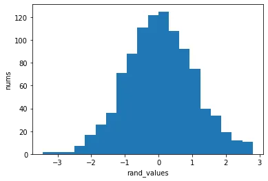
rand_values = [np.random.normal(loc=0.0) for _ in range(1000)]
_ = plt.hist(rand_values, bins=20)
_ = plt.xlabel("rand_values")
_ = plt.ylabel("nums")

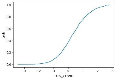
cdf = get_discrete_cdf(rand_values)

x_p = list(zip(rand_values, cdf))
x_p.sort(key=lambda it: it[0])

x = [it[0] for it in x_p]
y = [it[1] for it in x_p]

_ = plt.plot(x, y)
_ = plt.xlabel("rand_values")
_ = plt.ylabel("prob")

- tttzof351