我希望创建一个直方图,比较三组数据。但是,我想通过每组内的总计数来标准化每个直方图,而不是通过总计数来标准化。下面是我的代码。
library(ggplot2)
library(reshape2)
# Creates dataset
set.seed(9)
df<- data.frame(values = c(runif(400,20,50),runif(300,40,80),runif(600,0,30)),labels = c(rep("med",400),rep("high",300),rep("low",600)))
levs <- c("low", "med", "high")
df$labels <- factor(df$labels, levels = levs)
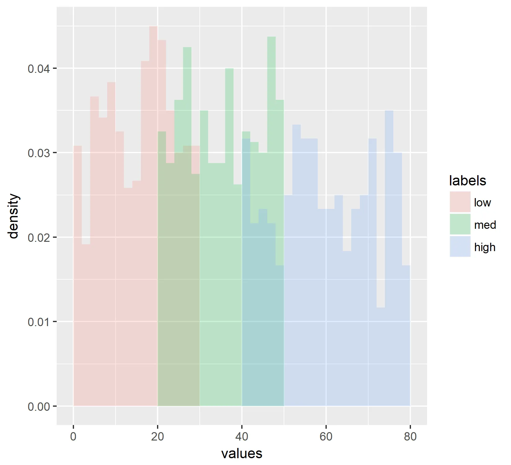
ggplot(df, aes(x=values, fill=labels)) +
geom_histogram(aes(y=..density..),
breaks= seq(0, 80, by = 2),
alpha=0.2,
position="identity")
生成一个直方图,看起来是按密度归一化的。
然而,我决定用手动验证密度的方法交叉检查这个密度图。为了做到这一点,我使用了以下代码:
# Separates the low medium and high groups
df1 <- df[df$labels == "low",]
df2 <- df[df$labels == "med",]
df3 <- df[df$labels == "high",]

# creates histogram for each group that is normalized by the total number of counts
hist_temp <- hist(df1$values, breaks=seq(0,80, by=2))
    tdf <- data.frame(hist_temp$breaks[2:length(hist_temp$breaks)],hist_temp$counts)
    colnames(tdf) <- c("bins","counts")
    tdf$norm <- tdf$counts/(sum(tdf$counts))
        low1 <- tdf

hist_temp <- hist(df2$values, breaks=seq(0,80, by=2))
    tdf <- data.frame(hist_temp$breaks[2:length(hist_temp$breaks)],hist_temp$counts)
    colnames(tdf) <- c("bins","counts")
    tdf$norm <- tdf$counts/(sum(tdf$counts))
        med1 <- tdf

hist_temp <- hist(df3$values, breaks=seq(0,80, by=2))
    tdf <- data.frame(hist_temp$breaks[2:length(hist_temp$breaks)],hist_temp$counts)
    colnames(tdf) <- c("bins","counts")
    tdf$norm <- tdf$counts/(sum(tdf$counts))
        high1 <- tdf

# Combines normalized histograms for each data frame and melts them into a single vector for plotting
Tdata <- data.frame(low1$bins,low1$norm,med1$norm,high1$norm)
    colnames(Tdata) <- c("bin","low", "med", "high")
    Tdata<- melt(Tdata,id = "bin")

levs <- c("low", "med", "high")
Tdata$variable <- factor(Tdata$variable, levels = levs)

# Plot the data
ggplot(Tdata, aes(group=variable, colour= variable)) +
    geom_line(aes(x = bin, y = value))
生成的图像如下所示:
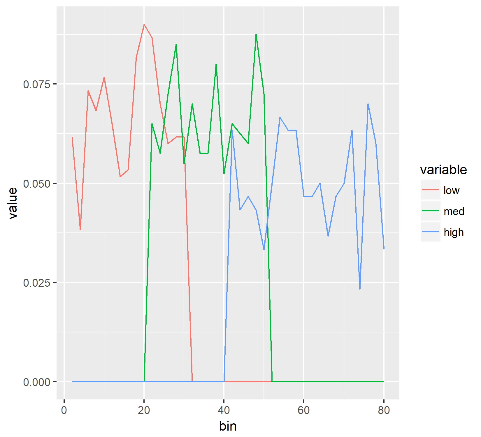
可以看到,这两个图像非常不同,我无法弄清楚为什么。 Y轴应该是相同的,但事实并非如此。因此,假设我没有犯任何愚蠢的数学错误,我认为希望直方图看起来像线图,但我无法找到一种方法实现这一点。任何帮助都将不胜感激,谢谢。
编辑以添加进一步的不起作用的示例:
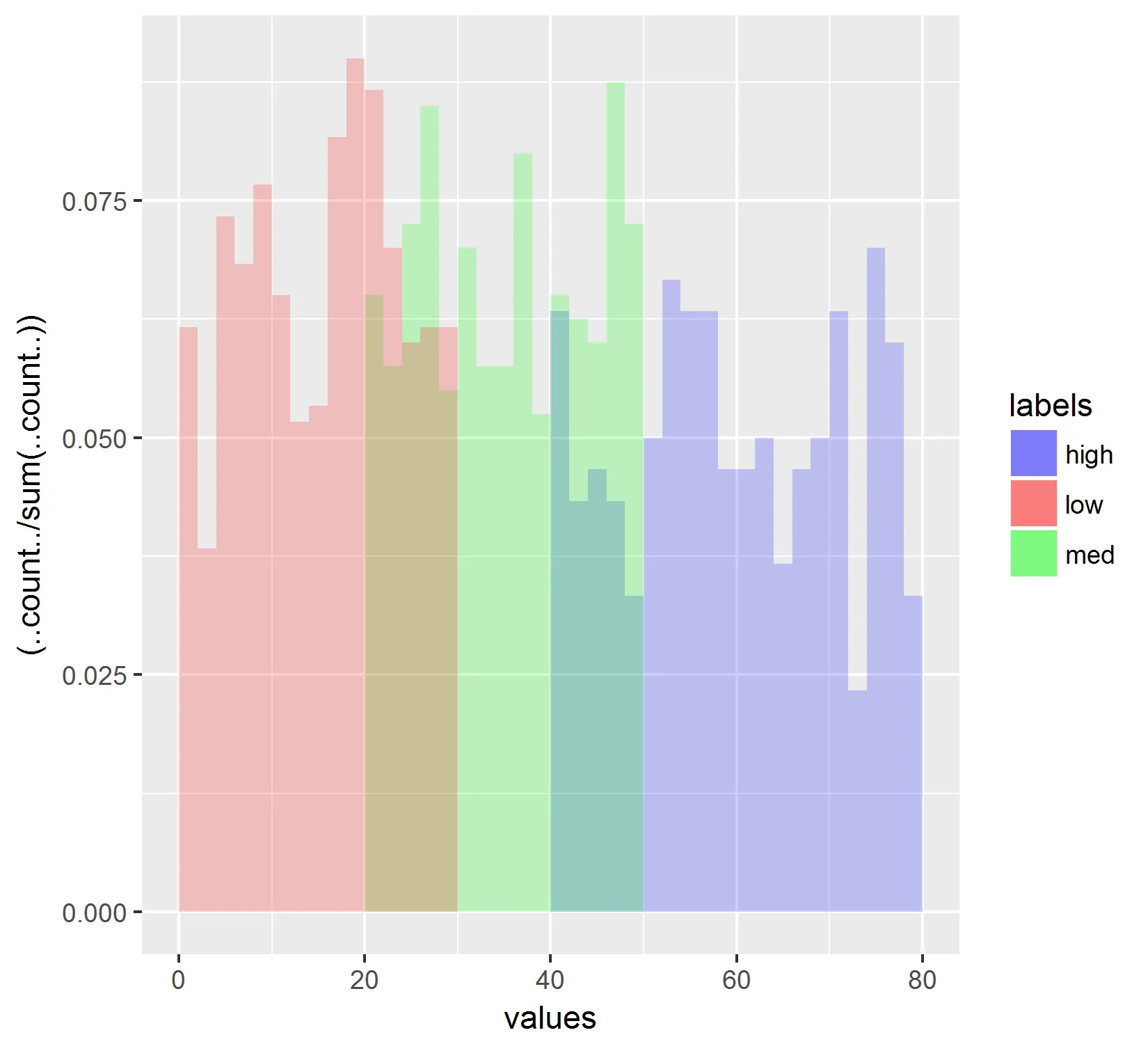
我还尝试使用代码中的..count../(sum(..count..))方法:
# Histogram where each histogram is divided by the total count of all groups
    ggplot(df, aes(x=values, fill=labels, group=labels)) +
        geom_histogram(aes(y=(..count../sum(..count..))),
                       breaks= seq(0, 80, by = 2),
                       alpha=0.2,
                       position="identity")
根据这些结果:
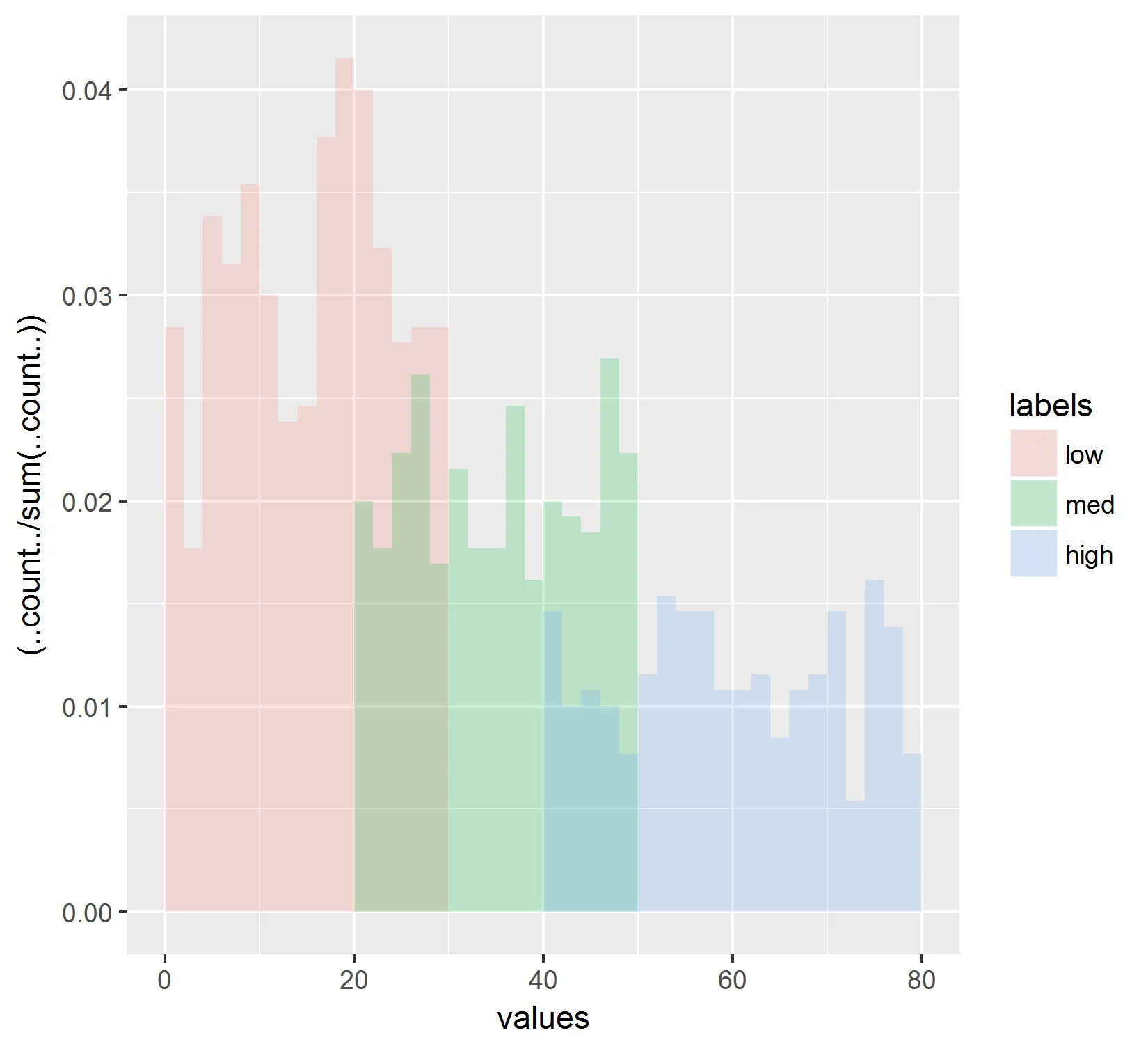 这只是将所有直方图的总计数归一化。这也不能反映出我在线图中看到的情况。此外,我尝试在分子、分母和分子和分母中替换..count..为..ncount..,但也无法重新创建线图中显示的结果。
此外,我尝试使用“position=stack”而不是使用下面的标识代码:
    ggplot(df, aes(x=values, fill=labels, group=labels)) +
        geom_histogram(aes(y=..density..),
                       breaks= seq(0, 80, by = 2),
                       alpha=0.2,
                       position="stack")
我得到了以下结果:
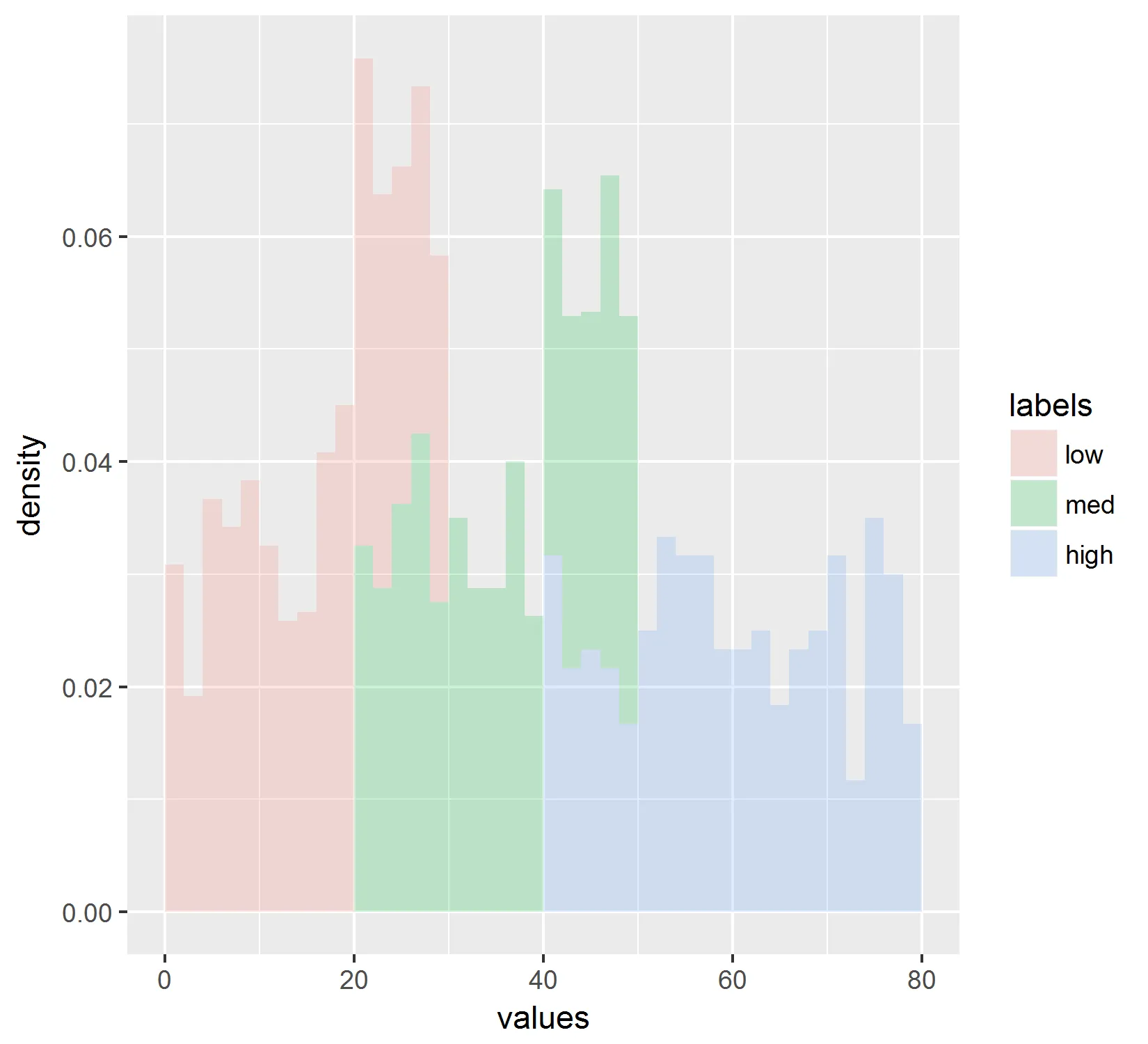 但是这并不反映折线图中显示的值。
取得了进展!使用Joran在这篇帖子中概述的方法,我现在可以生成与折线图相同的直方图。以下是代码:
# Plot where each histogram is normalized by its own counts.
ggplot(df,aes(x=values, fill=labels, group=labels)) +
    geom_histogram(data=subset(df, labels == 'high'),
                   aes(y=(..count../sum(..count..))),
                   breaks= seq(0, 80, by = 2),
                   alpha = 0.2) +
    geom_histogram(data=subset(df, labels == 'med'),
                   aes(y=(..count../sum(..count..))),
                   breaks= seq(0, 80, by = 2),
                   alpha = 0.2) +
    geom_histogram(data=subset(df, labels == 'low'),
                   aes(y=(..count../sum(..count..))),
                   breaks= seq(0, 80, by = 2),
                   alpha = 0.2) +
    scale_fill_manual(values = c("blue","red","green"))
这将生成以下图表:
 然而,我仍然无法重新排列数据,以便图例按照“低”,“中”,“高”的顺序显示,而不是按字母顺序显示。我已经设置了因子的级别。(请参见第一个代码块)。 有什么想法吗?
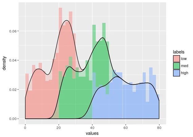
foreach是正确的方法,但是现在我没有时间去处理它。你应该试试看:D - Vitor Bianchi Lanzetta