2016年4月6日更新
在大多数情况下,正确获取拟合参数的错误是微妙的。
让我们考虑拟合一个函数y=f(x),其中您有一组数据点(x_i, y_i, yerr_i),其中i是在每个数据点上运行的索引。
在大多数物理测量中,误差yerr_i是测量设备或过程的系统性不确定度,因此可以将其视为不依赖于i的常数。
使用哪种拟合函数以及如何获取参数错误?
optimize.leastsq方法将返回分数协方差矩阵。 将该矩阵的所有元素乘以残差方差(即减少的卡方)并取对角线元素的平方根,将给您提供拟合参数标准偏差的估计。 我已经在下面的一个函数中包含了执行该操作的代码。
另一方面,如果使用optimize.curvefit,上述过程的第一部分(乘以减少的卡方)将在幕后为您完成。 然后,您需要取协方差矩阵的对角线元素的平方根,以获得拟合参数标准偏差的估计。
此外,optimize.curvefit提供了可选参数来处理更一般的情况,其中yerr_i值对每个数据点都不同。 来自文档:
sigma : None or M-length sequence, optional
    If not None, the uncertainties in the ydata array. These are used as
    weights in the least-squares problem
    i.e. minimising ``np.sum( ((f(xdata, *popt) - ydata) / sigma)**2 )``
    If None, the uncertainties are assumed to be 1.

absolute_sigma : bool, optional
    If False, `sigma` denotes relative weights of the data points.
    The returned covariance matrix `pcov` is based on *estimated*
    errors in the data, and is not affected by the overall
    magnitude of the values in `sigma`. Only the relative
    magnitudes of the `sigma` values matter.
如何确定我的误差是正确的?
确定拟合参数的标准误差的适当估计是一个复杂的统计问题。实际上,optimize.curvefit和optimize.leastsq实现的协方差矩阵的结果取决于关于误差的概率分布和参数之间的相互作用的假设; 这些相互作用可能存在于您特定的拟合函数f(x)中。
在我看来,处理复杂的f(x)的最佳方法是使用引导法,该方法在此链接中概述。
让我们看一些例子
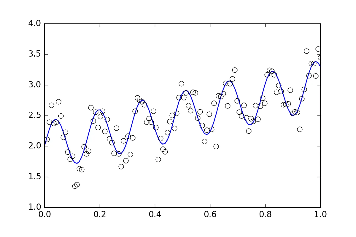
首先是一些样板代码。让我们定义一个波浪线函数并生成带有随机误差的数据集。 我们将生成一个带有小随机误差的数据集。
import numpy as np
from scipy import optimize
import random
def f( x, p0, p1, p2):
return p0*x + 0.4*np.sin(p1*x) + p2
def ff(x, p):
return f(x, *p)
p0 = 1.0
p1 = 40
p2 = 2.0
pstart = [
p0 + random.random(),
p1 + 5.*random.random(),
p2 + random.random()
]
%matplotlib inline
import matplotlib.pyplot as plt
xvals = np.linspace(0., 1, 120)
yvals = f(xvals, p0, p1, p2)
xdata = np.array(xvals)
np.random.seed(42)
err_stdev = 0.2
yvals_err = np.random.normal(0., err_stdev, len(xdata))
ydata = f(xdata, p0, p1, p2) + yvals_err
plt.plot(xvals, yvals)
plt.plot(xdata, ydata, 'o', mfc='None')
现在,让我们使用各种可用的方法来拟合函数:
`optimize.leastsq`
def fit_leastsq(p0, datax, datay, function):

    errfunc = lambda p, x, y: function(x,p) - y

    pfit, pcov, infodict, errmsg, success = \
        optimize.leastsq(errfunc, p0, args=(datax, datay), \
                          full_output=1, epsfcn=0.0001)

    if (len(datay) > len(p0)) and pcov is not None:
        s_sq = (errfunc(pfit, datax, datay)**2).sum()/(len(datay)-len(p0))
        pcov = pcov * s_sq
    else:
        pcov = np.inf

    error = []
    for i in range(len(pfit)):
        try:
          error.append(np.absolute(pcov[i][i])**0.5)
        except:
          error.append( 0.00 )
    pfit_leastsq = pfit
    perr_leastsq = np.array(error)
    return pfit_leastsq, perr_leastsq

pfit, perr = fit_leastsq(pstart, xdata, ydata, ff)

print("\n# Fit parameters and parameter errors from lestsq method :")
print("pfit = ", pfit)
print("perr = ", perr)
pfit = [ 1.04951642 39.98832634 1.95947613]
perr = [ 0.0584024 0.10597135 0.03376631]
`optimize.curve_fit`
def fit_curvefit(p0, datax, datay, function, yerr=err_stdev, **kwargs):
    """
    Note: As per the current documentation (Scipy V1.1.0), sigma (yerr) must be:
        None or M-length sequence or MxM array, optional
    Therefore, replace:
        err_stdev = 0.2
    With:
        err_stdev = [0.2 for item in xdata]
    Or similar, to create an M-length sequence for this example.
    """
    pfit, pcov = \
         optimize.curve_fit(f,datax,datay,p0=p0,\
                            sigma=yerr, epsfcn=0.0001, **kwargs)
    error = []
    for i in range(len(pfit)):
        try:
          error.append(np.absolute(pcov[i][i])**0.5)
        except:
          error.append( 0.00 )
    pfit_curvefit = pfit
    perr_curvefit = np.array(error)
    return pfit_curvefit, perr_curvefit

pfit, perr = fit_curvefit(pstart, xdata, ydata, ff)

print("\n# Fit parameters and parameter errors from curve_fit method :")
print("pfit = ", pfit)
print("perr = ", perr)
pfit = [ 1.04951642 39.98832634 1.95947613]
perr = [ 0.0584024 0.10597135 0.03376631]
`Bootstrap`
def fit_bootstrap(p0, datax, datay, function, yerr_systematic=0.0):
errfunc = lambda p, x, y: function(x,p) - y
pfit, perr = optimize.leastsq(errfunc, p0, args=(datax, datay), full_output=0)
residuals = errfunc(pfit, datax, datay)
sigma_res = np.std(residuals)
sigma_err_total = np.sqrt(sigma_res**2 + yerr_systematic**2)
ps = []
for i in range(100):
randomDelta = np.random.normal(0., sigma_err_total, len(datay))
randomdataY = datay + randomDelta
randomfit, randomcov = \
optimize.leastsq(errfunc, p0, args=(datax, randomdataY),\
full_output=0)
ps.append(randomfit)
ps = np.array(ps)
mean_pfit = np.mean(ps,0)
Nsigma = 1.
err_pfit = Nsigma * np.std(ps,0)
pfit_bootstrap = mean_pfit
perr_bootstrap = err_pfit
return pfit_bootstrap, perr_bootstrap
pfit, perr = fit_bootstrap(pstart, xdata, ydata, ff)
print("\n# Fit parameters and parameter errors from bootstrap method :")
print("pfit = ", pfit)
print("perr = ", perr)
pfit = [ 1.05058465 39.96530055 1.96074046]
perr = [ 0.06462981 0.1118803 0.03544364]
观察结果
我们已经开始看到一些有趣的事情了,所有三种方法的参数和误差估计几乎是一致的。这是好的!
现在,假设我们想告诉拟合函数,我们的数据存在一些其他的不确定性,比如系统误差,它会导致额外的误差是err_stdev值的二十倍。那是非常大的误差,实际上,如果我们使用这种误差模拟一些数据,那么看起来就像这样:
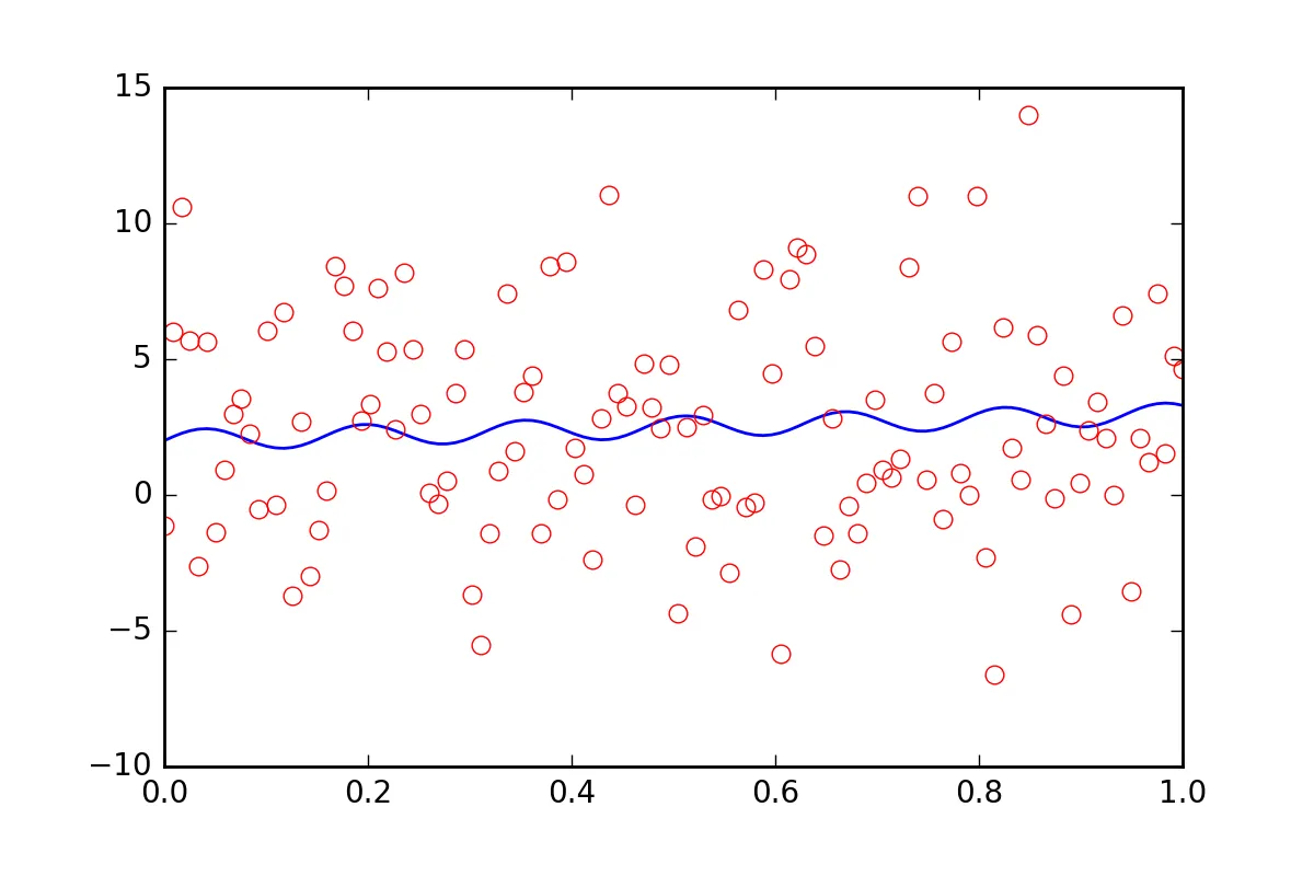
显然,我们不可能恢复具有这种噪声级别的拟合参数。
首先,让我们认识到leastsq甚至不允许我们输入这个新的系统误差信息。让我们看看当我们告诉curve_fit有关误差时它会做什么:
pfit, perr = fit_curvefit(pstart, xdata, ydata, ff, yerr=20*err_stdev)

print("\nFit parameters and parameter errors from curve_fit method (20x error) :")
print("pfit = ", pfit)
print("perr = ", perr)
Fit parameters and parameter errors from curve_fit method (20x error) :
pfit =  [  1.04951642  39.98832633   1.95947613]
perr =  [ 0.0584024   0.10597135  0.03376631]
咦?这一定是错的!
虽然过去这就是故事的结尾,但最近 curve_fit 添加了一个可选参数 absolute_sigma:
pfit, perr = fit_curvefit(pstart, xdata, ydata, ff, yerr=20*err_stdev, absolute_sigma=True)

print("\n# Fit parameters and parameter errors from curve_fit method (20x error, absolute_sigma) :")
print("pfit = ", pfit)
print("perr = ", perr)
pfit = [ 1.04951642 39.98832633 1.95947613]
perr = [ 1.25570187 2.27847504 0.72600466]
这有点好了一些,但仍然有点可疑。curve_fit认为我们可以从那个嘈杂的信号中得到一个拟合,p1参数的误差水平为10%。让我们看看bootstrap有什么说法:
pfit, perr = fit_bootstrap(pstart, xdata, ydata, ff, yerr_systematic=20.0)

print("\nFit parameters and parameter errors from bootstrap method (20x error):")
print("pfit = ", pfit)
print("perr = ", perr)
Fit parameters and parameter errors from bootstrap method (20x error):
pfit =  [  2.54029171e-02   3.84313695e+01   2.55729825e+00]
perr =  [  6.41602813  13.22283345   3.6629705 ]
啊,那或许是我们拟合参数误差的更好估计。 bootstrap 认为对于 p1 其不确定性约为 34%。
总结
optimize.leastsq 和 optimize.curvefit 提供了一种估算拟合参数误差的方式,但我们不能盲目使用这些方法而不加质疑。 bootstrap 是一种使用暴力方法的统计学方法,我认为它在较难解释的情况下更容易发挥作用。
我强烈建议针对特定问题尝试使用 curvefit 和 bootstrap。如果它们相似,那么 curvefit 计算成本更低,因此可能值得使用。 如果它们有显著不同,那么我会选择使用 bootstrap。