如何使用Python确定拟合参数的不确定性？

Question

我有以下 x 和 y 的数据:

x   y
1.71    0.0
1.76    5.0
1.81    10.0
1.86    15.0
1.93    20.0
2.01    25.0
2.09    30.0
2.20    35.0
2.32    40.0
2.47    45.0
2.65    50.0
2.87    55.0
3.16    60.0
3.53    65.0
4.02    70.0
4.69    75.0
5.64    80.0
7.07    85.0
9.35    90.0
13.34   95.0
21.43   100.0

对于上述数据，我试图将其拟合成以下形式：

然而，x和y存在一定的不确定性，其中x的不确定度为x的50％，y具有固定的不确定性。 我正在尝试使用uncertainties库来确定拟合参数的不确定性。但是，我在使用scipy optimize的curve_fit函数进行曲线拟合时遇到了问题。 我收到以下错误：

minpack.error: Result from function call is not a proper array of floats.

我该如何解决此错误并确定拟合参数（a，b和n）的不确定性？

MWE

from __future__ import division
import numpy as np
import re
from scipy import optimize, interpolate, spatial
from scipy.interpolate import UnivariateSpline
from uncertainties import unumpy


def linear_fit(x, a, b):
    return a * x + b


uncertainty = 0.5
y_error = 1.2
x = np.array([1.71, 1.76, 1.81, 1.86, 1.93, 2.01, 2.09, 2.20, 2.32, 2.47, 2.65, 2.87, 3.16, 3.53, 4.02, 4.69, 5.64, 7.07, 9.35, 13.34, 21.43])
x_uncertainty = x * uncertainty
x = unumpy.uarray(x, x_uncertainty)
y = np.array([0.0, 5.0, 10.0, 15.0, 20.0, 25.0, 30.0, 35.0, 40.0, 45.0, 50.0, 55.0, 60.0, 65.0, 70.0, 75.0, 80.0, 85.0, 90.0, 95.0, 100.0])
y = unumpy.uarray(y, y_error)


n = np.arange(0, 5, 0.005)
coefficient_determination_on = np.empty(shape = (len(n),))
for j in range(len(n)):
    n_correlation = n[j]
    x_fit = 1 / ((x) ** n_correlation)
    y_fit = y
    fit_a_raw, fit_b_raw = optimize.curve_fit(linear_fit, x_fit, y_fit)[0]
    x_prediction = (fit_a_raw / ((x) ** n_correlation)) + fit_b_raw
    y_residual_squares = np.sum((x_prediction - y) ** 2)
    y_total_squares = np.sum((y - np.mean(y)) ** 2)
    coefficient_determination_on[j] = 1 - (y_residual_squares / y_total_squares)

- Tom Kurushingal

---

我认为scipy的optimize.curve_fit方法没有实现接受unumpy数组。对于这种拟合，您最好使用scikit-learn并使用指数点积（用于实际回归）和白噪声（用于不确定性）内核进行高斯过程回归。我不是专家-尝试一下，如果有问题，请使用scikit-learn标记提问。 - Daniel F

浏览文档（很棒的包！），您可能能够使用uncertainties.wrap与optimize.curve_fit一起工作，但这似乎需要奇迹。不过，为了测试这个问题，改变我在工作中的本地环境是我不愿意经历的痛苦。 - Daniel F

“uncertainties”似乎具有导数和矩阵逆函数，因此实现自己的非线性回归算法应该是可能的。虽然不如“scikit”快，但它应该能够工作。 - Daniel F

@DanielF 不确定我是否理解正确，但高斯过程是否允许在x或仅在y中添加附加误差？ 如果是，它在哪里设置？ - mikuszefski

你确定x的50%吗？这些小步骤是单调的事实有点矛盾。请注意，y值在25左右的值基本上可以是1到3之间的任何值，但增长大约为5%至10%。如果有50%的误差，这种单调行为应该会被噪声淹没。 - mikuszefski

请注意，对于您的数据，您应该有 x= a*y**n+b 而不是 y= a*x**n+b。在后者中，您没有一个适当的截距。它看起来确实是 (x-x0)**(1/n) 类型的。顺便问一下，n 应该是整数还是反过来看是整数根？ - mikuszefski

Answer 1

首先，我要说明的是，如果你想解决 a、b 和 n 的问题，这个问题是不可能“好好”地解决的。因为对于一个固定的 n，你的问题可以采用封闭形式的解决方案，但如果你让 n 自由变化，它就没有了，实际上这个问题可能有多个解。因此，传统的误差分析（如 uncertanities 使用的方法）会失效，你必须采用其他方法。

当 n 固定时

如果 n 是固定的，那么你的问题是调用的库不支持 uarray，所以你需要找到一种解决方法。幸运的是，线性拟合（在 l2 距离下）就是线性最小二乘法，它有一个封闭形式的解决方案，只需要用1来填充值，然后解决正规方程即可。

其中：

你可以这样做：

import numpy as np
from uncertainties import unumpy

uncertainty = 0.5
y_error = 1.2
n = 1.0

# Define x and y
x = np.array([1.71, 1.76, 1.81, 1.86, 1.93, 2.01, 2.09, 2.20, 2.32, 2.47, 2.65,
              2.87, 3.16, 3.53, 4.02, 4.69, 5.64, 7.07, 9.35, 13.34, 21.43])
# Take power of x values according to n
x_pow = x ** n
x_uncertainty = x_pow * uncertainty
x_fit = unumpy.uarray(np.c_[x_pow, np.ones_like(x)],
                      np.c_[x_uncertainty, np.zeros_like(x_uncertainty)])

y = np.array([0.0, 5.0, 10.0, 15.0, 20.0, 25.0, 30.0, 35.0, 40.0, 45.0, 50.0,
              55.0, 60.0, 65.0, 70.0, 75.0, 80.0, 85.0, 90.0, 95.0, 100.0])
y_fit = unumpy.uarray(y, y_error)

# Use normal equations to find coefficients
inv_mat = unumpy.ulinalg.pinv(x_fit.T.dot(x_fit))
fit_a, fit_b = inv_mat.dot(x_fit.T.dot(y_fit))

print('fit_a={}, fit_b={}'.format(fit_a, fit_b))

结果：

fit_a=4.8+/-2.6, fit_b=28+/-10

未知的情况 n

如果存在未知的情况 n，那么您可能会遇到一些麻烦，因为问题是非凸的。在这种情况下，线性误差分析（由uncertainties执行）将不起作用。

一种解决方案是使用一些软件包（如pymc）执行贝叶斯推断。如果您对此感兴趣，我可以尝试写一篇文章，但它可能没有上面的内容清晰。

- Jonas Adler

---

关于缺乏uarray支持uncertanties.wrap()可能可以解决问题。更好的是，直接通过unumpy支持numpy。 - Tobias Kienzler

我看到 OP 已经使用了 uarray，并且 wrap 也被提到过（尽管似乎没有被任何人进一步追究）。 - Tobias Kienzler

Answer 2

在跟踪线性函数的案例后，我认为可以采用类似的方法。不过，解决拉格朗日问题似乎非常繁琐，当然也是可能的。我想出了一种似乎合理且应该能够得到非常相似结果的不同测量方法。我重新调整误差椭圆，使其成为一个切点。我以这个接触点(X_k,Y_k)到距离作为卡方的度量，它是从(x_k-X_k/sx_k)**2+(y_k-Y_k/sy_k)**2计算出来的。因为在纯y误差的情况下，这是标准的最小二乘拟合。对于纯x误差，它只是反过来。对于等于的x,y误差，它将给出垂直规则，即最短距离。使用相应的卡方函数scipy.optimize.leastsq已经提供了从Hesse近似的协方差矩阵。但需要注意的是，参数之间存在强相关性。

我的过程如下:

import matplotlib
matplotlib.use('Qt5Agg')

import matplotlib.pyplot as plt
import numpy as np
import myModules.multipoleMoments as mm 
from random import random
from scipy.optimize import minimize,leastsq


###for gaussion distributed errors
def boxmuller(x0,sigma):
    u1=random()
    u2=random()
    ll=np.sqrt(-2*np.log(u1))
    z0=ll*np.cos(2*np.pi*u2)
    z1=ll*np.cos(2*np.pi*u2)
    return sigma*z0+x0, sigma*z1+x0


###function to fit
def f(t,c,d,n):
    return c+d*np.abs(t)**n


###to create some test data
def test_data(c,d,n, xList,const_sx,rel_sx,const_sy,rel_sy):
    yList=[f(t,c,d,n) for t in xList]
    xErrList=[ boxmuller(x,const_sx+x*rel_sx)[0] for x in xList]
    yErrList=[ boxmuller(y,const_sy+y*rel_sy)[0] for y in yList]
    return xErrList,yErrList


###how to rescale the ellipse to make fitfunction a tangent
def elliptic_rescale(x,c,d,n,x0,y0,sa,sb):
    y=f(x,c,d,n)
    r=np.sqrt((x-x0)**2+(y-y0)**2)
    kappa=float(sa)/float(sb)
    tau=np.arctan2(y-y0,x-x0)
    new_a=r*np.sqrt(np.cos(tau)**2+(kappa*np.sin(tau))**2)
    return new_a


###for plotting ellipses
def ell_data(a,b,x0=0,y0=0):
    tList=np.linspace(0,2*np.pi,150)
    k=float(a)/float(b)
    rList=[a/np.sqrt((np.cos(t))**2+(k*np.sin(t))**2) for t in tList]
    xyList=np.array([[x0+r*np.cos(t),y0+r*np.sin(t)] for t,r in zip(tList,rList)])
    return xyList


###residual function to calculate chi-square
def residuals(parameters,dataPoint):#data point is (x,y,sx,sy)
    c,d,n= parameters
    theData=np.array(dataPoint)
    best_t_List=[]
    for i in range(len(dataPoint)):
        x,y,sx,sy=dataPoint[i][0],dataPoint[i][1],dataPoint[i][2],dataPoint[i][3]
        ###getthe point on the graph where it is tangent to an error-ellipse
        ed_fit=minimize(elliptic_rescale,0,args=(c,d,n,x,y,sx,sy) )
        best_t=ed_fit['x'][0]
        best_t_List+=[best_t]
    best_y_List=[f(t,c,d,n) for t in best_t_List]
    ##weighted distance not squared yet, as this is done by scipy.optimize.leastsq
    wighted_dx_List=[(x_b-x_f)/sx for x_b,x_f,sx in zip( best_t_List,theData[:,0], theData[:,2] ) ]
    wighted_dy_List=[(x_b-x_f)/sx for x_b,x_f,sx in zip( best_y_List,theData[:,1], theData[:,3] ) ]
    return wighted_dx_List+wighted_dy_List


###some start values
cc,dd,nn=2.177,.735,1.75
ssaa,ssbb=1,3
xx0,yy0=2,3
csx,rsx=.1,.05
csy,rsy=.4,.00

####some data
xThData=np.linspace(0,3,15)
yThData=[ f(t, cc,dd,nn) for t in xThData]

###some noisy data
xNoiseData,yNoiseData=test_data(cc,dd,nn, xThData, csx,rsx, csy,rsy)
xGuessdError=[csx+rsx*x for x in xNoiseData]
yGuessdError=[csy+rsy*y for y in yNoiseData]

###plot that
fig1 = plt.figure(1)
ax=fig1.add_subplot(1,1,1)
ax.plot(xThData,yThData)
ax.errorbar(xNoiseData,yNoiseData, xerr=xGuessdError, yerr=yGuessdError, fmt='none',ecolor='r')

#### and plot...
for i in range(len(xNoiseData)):
    ###...an elliple on the error values
    el0=ell_data(xGuessdError[i],yGuessdError[i],x0=xNoiseData[i],y0=yNoiseData[i])
    ax.plot(*zip(*el0),linewidth=1, color="#808080",linestyle='-')
    ####...as well as a scaled version that touches the original graph. This gives the error shortest distance to that graph
    ed_fit=minimize(elliptic_rescale,0,args=(cc,dd,nn,xNoiseData[i],yNoiseData[i],xGuessdError[i],yGuessdError[i]) )
    best_t=ed_fit['x'][0]
    best_a=elliptic_rescale(best_t,cc,dd,nn,xNoiseData[i],yNoiseData[i],xGuessdError[i],yGuessdError[i])
    el0=ell_data(best_a,best_a/xGuessdError[i]*yGuessdError[i],x0=xNoiseData[i],y0=yNoiseData[i])
    ax.plot(*zip(*el0),linewidth=1, color="#a000a0",linestyle='-')

###Now fitting
zipData=zip(xNoiseData,yNoiseData, xGuessdError, yGuessdError)    
estimate = [2.0,1,2.5]
bestFitValues, cov,info,mesg, ier = leastsq(residuals, estimate,args=(zipData), full_output=1)
print bestFitValues
####covariance matrix
####note e.g.: https://dev59.com/kWUq5IYBdhLWcg3wBL7j
s_sq = (np.array(residuals(bestFitValues, zipData))**2).sum()/(len(zipData)-len(estimate))
pcov = cov * s_sq
print pcov



#### and plot the result...
ax.plot(xThData,[f(x,*bestFitValues) for x in xThData])
for i in range(len(xNoiseData)):
    ####...as well as a scaled ellipses that touches the fitted graph. 
    ed_fit=minimize(elliptic_rescale,0,args=(bestFitValues[0],bestFitValues[1],bestFitValues[2],xNoiseData[i],yNoiseData[i],xGuessdError[i],yGuessdError[i]) )
    best_t=ed_fit['x'][0]
    best_a=elliptic_rescale(best_t,bestFitValues[0],bestFitValues[1],bestFitValues[2],xNoiseData[i],yNoiseData[i],xGuessdError[i],yGuessdError[i])
    el0=ell_data(best_a,best_a/xGuessdError[i]*yGuessdError[i],x0=xNoiseData[i],y0=yNoiseData[i])
    ax.plot(*zip(*el0),linewidth=1, color="#f0a000",linestyle='-')

#~ ax.grid(None)
plt.show()

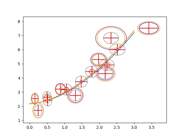蓝色曲线是原始函数。红色误差条数据点是由此计算出来的。灰色椭圆显示“常数概率密度线”。紫色椭圆以原始图形为切线，橙色椭圆以拟合为切线。

这里的最佳拟合值是（不是您的数据！）：

[ 2.16146783  0.80204967  1.69951865]

协方差矩阵的形式为：

[[ 0.0644794  -0.05418743  0.05454876]
 [-0.05418743  0.07228771 -0.08172885]
 [ 0.05454876 -0.08172885  0.10173394]]

编辑 关于“椭圆距离”，我认为这正是所链接论文中的拉格朗日方法所做的。只是对于直线，你可以写出一个精确解，而在这种情况下你不能。

更新 我遇到了一些与OP数据有关的问题。不过通过重新缩放，它可以工作。由于斜率和指数高度相关，因此我首先必须弄清楚协方差矩阵如何针对重新缩放的数据发生变化。详细信息可以在J. Phys. Chem. 105 (2001) 3917中找到。

使用上面的函数定义，数据处理将如下所示：

###some start values
cc,dd,nn=.2,1,7.5
csx,rsx=2.0,.0
csy,rsy=0,.5

###some noisy data
yNoiseData=np.array([1.71,1.76, 1.81, 1.86, 1.93, 2.01, 2.09, 2.20, 2.32, 2.47, 2.65, 2.87, 3.16, 3.53, 4.02, 4.69, 5.64, 7.07, 9.35,13.34,21.43])
xNoiseData=np.array([0.0,5.0,10.0,15.0,20.0,25.0,30.0,35.0,40.0,45.0,50.0,55.0,60.0,65.0,70.0,75.0,80.0,85.0,90.0,95.0,100.0])

xGuessdError=[csx+rsx*x for x in xNoiseData]
yGuessdError=[csy+rsy*y for y in yNoiseData]

###plot that
fig1 = plt.figure(1)
ax=fig1.add_subplot(1,2,2)
bx=fig1.add_subplot(1,2,1)
ax.errorbar(xNoiseData,yNoiseData, xerr=xGuessdError, yerr=yGuessdError, fmt='none',ecolor='r')

####rescaling        

print "\n++++++++++++++++++++++++  scaled ++++++++++++++++++++++++\n"
alpha=.05
beta=.01
xNoiseDataS   = [   beta*x for x in   xNoiseData   ]
yNoiseDataS   = [   alpha*x for x in   yNoiseData   ]
xGuessdErrorS  = [   beta*x for x in   xGuessdError ]
yGuessdErrorS  = [   alpha*x for x in   yGuessdError ] 


xtmp=np.linspace(0,1.1,25)
bx.errorbar(xNoiseDataS,yNoiseDataS, xerr=xGuessdErrorS, yerr=yGuessdErrorS, fmt='none',ecolor='r')


###Now fitting
zipData=zip(xNoiseDataS,yNoiseDataS, xGuessdErrorS, yGuessdErrorS)
estimate = [.1,1,7.5]
bestFitValues, cov,info,mesg, ier = leastsq(residuals, estimate,args=(zipData), full_output=1)
print bestFitValues
plt.plot(xtmp,[ f(x,*bestFitValues)for x in xtmp])
####covariance matrix
s_sq = (np.array(residuals(bestFitValues, zipData))**2).sum()/(len(zipData)-len(estimate))
pcov = cov * s_sq
print pcov

#### scale back  
print "\n++++++++++++++++++++++++  scaled back ++++++++++++++++++++++++\n"


realBestFitValues= [bestFitValues[0]/alpha, bestFitValues[1]/alpha*(beta)**bestFitValues[2],bestFitValues[2] ]
print realBestFitValues
uMX = np.array( [[1/alpha,0,0],[0,beta**bestFitValues[2]/alpha,bestFitValues[1]/alpha*beta**bestFitValues[2]*np.log(beta)],[0,0,1]] )
uMX_T = uMX.transpose()
realCov = np.dot(uMX, np.dot(pcov,uMX_T))
print realCov

for i,para in enumerate(["b","a","n"]):
    print para+" = "+"{:.2e}".format(realBestFitValues[i])+" +/- "+"{:.2e}".format(np.sqrt(realCov[i,i]))

ax.plot(xNoiseData,[f(x,*realBestFitValues) for x in xNoiseData])

plt.show()

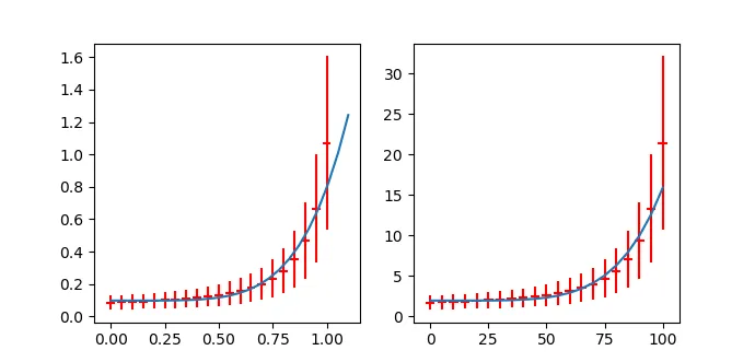
因此，数据已经被合理拟合。然而，我认为还有一个线性项。

输出结果如下：

++++++++++++++++++++++++  scaled ++++++++++++++++++++++++

[ 0.09788886  0.69614911  5.2221032 ]
[[  1.25914194e-05   2.86541696e-05   6.03957467e-04]
 [  2.86541696e-05   3.88675025e-03   2.00199108e-02]
 [  6.03957467e-04   2.00199108e-02   1.75756532e-01]]

++++++++++++++++++++++++  scaled back ++++++++++++++++++++++++

[1.9577772055183396, 5.0064036934715239e-10, 5.2221031993990517]
[[  5.03656777e-03  -2.74367539e-11   1.20791493e-02]
 [ -2.74367539e-11   8.69854174e-19  -3.90815222e-10]
 [  1.20791493e-02  -3.90815222e-10   1.75756532e-01]]

b = 1.96e+00 +/- 7.10e-02
a = 5.01e-10 +/- 9.33e-10
n = 5.22e+00 +/- 4.19e-01

可以看到协方差矩阵中斜率和指数之间有很强的相关性。同时请注意，斜率的误差非常大。

顺便说一句 使用模型b+a*x**n + e*x，我得到了。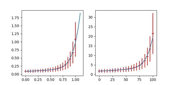

++++++++++++++++++++++++  scaled ++++++++++++++++++++++++

[ 0.08050174  0.78438855  8.11845402  0.09581568]
[[  5.96210962e-06   3.07651631e-08  -3.57876577e-04  -1.75228231e-05]
 [  3.07651631e-08   1.39368435e-03   9.85025139e-03   1.83780053e-05]
 [ -3.57876577e-04   9.85025139e-03   1.85226736e-01   2.26973118e-03]
 [ -1.75228231e-05   1.83780053e-05   2.26973118e-03   7.92853339e-05]]

++++++++++++++++++++++++  scaled back ++++++++++++++++++++++++

[1.6100348667765145, 9.0918698097511416e-16, 8.1184540175879985, 0.019163135651422442]
[[  2.38484385e-03   2.99690170e-17  -7.15753154e-03  -7.00912926e-05]
 [  2.99690170e-17   3.15340690e-30  -7.64119623e-16  -1.89639468e-18]
 [ -7.15753154e-03  -7.64119623e-16   1.85226736e-01   4.53946235e-04]
 [ -7.00912926e-05  -1.89639468e-18   4.53946235e-04   3.17141336e-06]]
b = 1.61e+00 +/- 4.88e-02
a = 9.09e-16 +/- 1.78e-15
n = 8.12e+00 +/- 4.30e-01
e = 1.92e-02 +/- 1.78e-03

当然，如果你添加参数，适合度会变得更好，但我认为这在这里看起来还算合理（甚至可能是b + a*x**n+e*x**m，但这太过深入了）。

- mikuszefski