scipy.stats.norm.fit是否有获取拟合参数误差的方法？

Question

我有一些数据，使用scipy.stats.normal对象的fit函数进行正态分布拟合，如下所示：

import numpy as np                                                                                                                                                                                                                       
import matplotlib.pyplot as plt                                                                                                                                                                                                          
from scipy.stats import norm                                                                                                                                                                                                             
import matplotlib.mlab as mlab                                                                                                                                                                                                           

x = np.random.normal(size=50000)                                                                                                                                                                                                         

fig, ax = plt.subplots()                                                                                                                                                                                                                 

nbins = 75                                                                                                                                                                                                                               
mu, sigma = norm.fit(x)                                                                                                                                                                                                                  
n, bins, patches = ax.hist(x,nbins,normed=1,facecolor = 'grey', alpha = 0.5, label='before');                                                                                                                                            
y0 = mlab.normpdf(bins, mu, sigma) # Line of best fit                                                                                                                                                                                    
ax.plot(bins,y0,'k--',linewidth = 2, label='fit before')                                                                                                                                                                                 
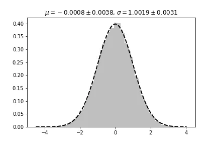
ax.set_title('$\mu$={}, $\sigma$={}'.format(mu, sigma))                                                                                                                                                                                  

plt.show()                                                                                                                                                                                                                               

我现在想提取拟合后的mu和sigma值中的不确定度/误差。我该怎么做？

- SomeRandomPhysicist

Answer 1

你可以使用 scipy.optimize.curve_fit 方法： 该方法不仅返回参数的估计最优值，还返回相应的协方差矩阵：

popt : 数组

使得 f(xdata, *popt) - ydata 的平方残差和最小的参数的最优值。

pcov : 2维数组

popt 的估计协方差。对角线提供了参数估计的方差。要计算参数的一个标准差误差，请使用 perr = np.sqrt(np.diag(pcov))。

如何 sigma 参数影响估计协方差取决于 absolute_sigma 参数，如上所述。

如果解处的雅可比矩阵没有满秩，则 “lm” 方法会返回一个填充有 np.inf 的矩阵，而“trf”和“dogbox”方法则使用摩尔-彭罗斯广义逆来计算协方差矩阵。

您可以根据协方差矩阵对角线元素的平方根计算参数的标准差误差，如下所示：

import numpy as np 
import matplotlib.pyplot as plt
from scipy.stats import norm 
from scipy.optimize import curve_fit

x = np.random.normal(size=50000)
fig, ax = plt.subplots() 
nbins = 75
n, bins, patches = ax.hist(x,nbins, density=True, facecolor = 'grey', alpha = 0.5, label='before'); 

centers = (0.5*(bins[1:]+bins[:-1]))
pars, cov = curve_fit(lambda x, mu, sig : norm.pdf(x, loc=mu, scale=sig), centers, n, p0=[0,1])

ax.plot(centers, norm.pdf(centers,*pars), 'k--',linewidth = 2, label='fit before') 
ax.set_title('$\mu={:.4f}\pm{:.4f}$, $\sigma={:.4f}\pm{:.4f}$'.format(pars[0],np.sqrt(cov[0,0]), pars[1], np.sqrt(cov[1,1 ])))

plt.show()

这将导致以下绘图结果：

- jdamp

---

请注意，这里报告的不确定性完全是由于将数据采样到75个箱中。除了任意分箱之外，没有噪声或非正态分布的来源。 - M Newville

@MNewville，那么norm.fit不会受到这些不确定性的影响吗？除了报告这些不确定性之外，curve_fit和norm.fit有什么不同？ - Always Learning Forever

@AlwaysLearningForever。我认为我之前的评论是不正确的——存在自然分布，并且使用足够多的箱子，质心和宽度的不确定性将稳定到非零值。至于norm.fit的作用：我不是100％确定，但我相信scipy.stats.norm.fit()使用Nelder-Mead进行拟合，而curve_fit使用Levenberg-Marquardt。我不知道scipy.stats.norm.fit()是否尝试估计不确定性，但我怀疑不会。 - M Newville

Answer 2

请参考lmfit (https://github.com/lmfit/lmfit-py)，该工具提供了更简单的界面，并报告拟合变量的不确定性。如果要将数据拟合到正态分布，则请参见http://lmfit.github.io/lmfit-py/builtin_models.html#example-1-fit-peak-data-to-gaussian-lorentzian-and-voigt-profiles，并使用类似以下的内容：

from lmfit.models import GaussianModel

model = GaussianModel()

# create parameters with initial guesses:
params = model.make_params(center=9, amplitude=40, sigma=1)  

result = model.fit(ydata, params, x=xdata)
print(result.fit_report())

报告将包括1-sigma误差，例如：

[[Variables]]
    sigma:       1.23218358 +/- 0.007374 (0.60%) (init= 1.0)
    center:      9.24277047 +/- 0.007374 (0.08%) (init= 9.0)
    amplitude:   30.3135620 +/- 0.157126 (0.52%) (init= 40.0)
    fwhm:        2.90157055 +/- 0.017366 (0.60%)  == '2.3548200*sigma'
    height:      9.81457817 +/- 0.050872 (0.52%)  == '0.3989423*amplitude/max(1.e-15, sigma)'

- M Newville

---

你在提供的示例代码中，是用什么方法确定初始参数值的？ - James Phillips

@JamesPhillips：我查看了数据（甚至没有在这里发布，但在lmfit示例中），并猜测了一下。Lmfit的GaussianModel实际上有一个“guess”方法来帮助猜测中心、振幅和sigma——链接的示例使用了该方法。Scipy或其他库中的峰值查找工具也可以用于识别峰值中心。但是：对于孤立的高斯峰，您不需要在初始猜测中那么接近，拟合就能收敛。 - M Newville

在这种情况下，你的猜测似乎很成功。 - James Phillips