在Python中拟合周期图形的方法：scipy.interpolate.splrep的参数，曲线方程？

Question

[原始问题]

我需要一个方程，根据以下数据，曲线随着时间的增长而无限增加。如何得到该方程？

[问题更新]

我需要为scipy.interpolate.splrep指定适当的参数。有人能帮忙吗？

此外，是否有一种方法可以从b样条系数中得到方程？

[备选问题]

如何使用Fourier级数分解获得拟合？

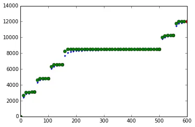
该图似乎是一个线性图的组合，一个周期函数pf1增加了四倍，一个更大的周期函数导致pf1无限地发生。这个问题被提出的原因是该图的困难。

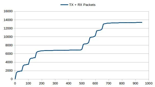
数据:

Time elapsed in sec.    TX + RX Packets
(0,0)
(10,2422)
(20,2902)
(30,2945)
(40,3059)
(50,3097)
(60,4332)
(70,4622)
(80,4708)
(90,4808)
(100,4841)
(110,6081)
(120,6333)
(130,6461)
(140,6561)
(150,6585)
(160,7673)
(170,8091)
(180,8210)
(190,8291)
(200,8338)
(210,8357)
(220,8357)
(230,8414)
(240,8414)
(250,8414)
(260,8414)
(270,8414)
(280,8414)
(290,8471)
(300,8471)
(310,8471)
(320,8471)
(330,8471)
(340,8471)
(350,8471)
(360,8471)
(370,8471)
(380,8471)
(390,8471)
(400,8471)
(410,8471)
(420,8528)
(430,8528)
(440,8528)
(450,8528)
(460,8528)
(470,8528)
(480,8528)
(490,8528)
(500,8528)
(510,9858)
(520,10029)
(530,10129)
(540,10224)
(550,10267)
(560,11440)
(570,11773)
(580,11868)
(590,11968)
(600,12039)
(610,13141)

我的代码：

import numpy as np
import matplotlib.pyplot as plt

points = np.array(
    [(0,0), (10,2422), (20,2902), (30,2945), (40,3059), (50,3097), (60,4332), (70,4622), (80,4708), (90,4808), (100,4841), (110,6081), (120,6333), (130,6461), (140,6561), (150,6585), (160,7673), (170,8091), (180,8210), (190,8291), (200,8338), (210,8357), (220,8357), (230,8414), (240,8414), (250,8414), (260,8414), (270,8414), (280,8414), (290,8471), (300,8471), (310,8471), (320,8471), (330,8471), (340,8471), (350,8471), (360,8471), (370,8471), (380,8471), (390,8471), (400,8471), (410,8471), (420,8528), (430,8528), (440,8528), (450,8528), (460,8528), (470,8528), (480,8528), (490,8528), (500,8528), (510,9858), (520,10029), (530,10129), (540,10224), (550,10267), (560,11440), (570,11773), (580,11868), (590,11968), (600,12039), (610,13141)]
    )
# get x and y vectors
x = points[:,0]
y = points[:,1]

# calculate polynomial
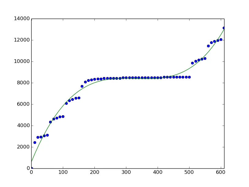
z = np.polyfit(x, y, 3)
print z
f = np.poly1d(z)

# calculate new x's and y's
x_new = np.linspace(x[0], x[-1], 50)
y_new = f(x_new)

plt.plot(x,y,'o', x_new, y_new)
plt.xlim([x[0]-1, x[-1] + 1 ])
plt.show()

我的输出：

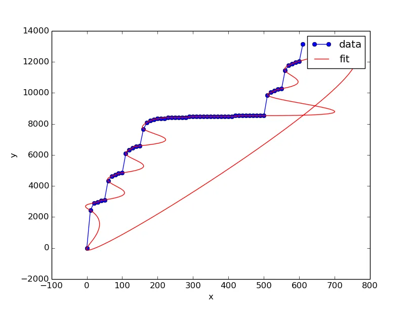
我的代码2：

import numpy as N
from scipy.interpolate import splprep, splev

x = N.array([0, 10, 20, 30, 40, 50, 60, 70, 80, 90, 100, 110, 120, 130, 140, 150, 160, 170, 180, 190, 200, 210, 220, 230, 240, 250, 260, 270, 280, 290, 300, 310, 320, 330, 340, 350, 360, 370, 380, 390, 400, 410, 420, 430, 440, 450, 460, 470, 480, 490, 500, 510, 520, 530, 540, 550, 560, 570, 580, 590, 600, 610])
y = N.array([0, 2422, 2902, 2945, 3059, 3097, 4332, 4622, 4708, 4808, 4841, 6081, 6333, 6461, 6561, 6585, 7673, 8091, 8210, 8291, 8338, 8357, 8357, 8414, 8414, 8414, 8414, 8414, 8414, 8471, 8471, 8471, 8471, 8471, 8471, 8471, 8471, 8471, 8471, 8471, 8471, 8471, 8528, 8528, 8528, 8528, 8528, 8528, 8528, 8528, 8528, 9858, 10029, 10129, 10224, 10267, 11440, 11773, 11868, 11968, 12039, 13141])

# spline parameters
s=1.0 # smoothness parameter
k=3 # spline order
nest=-1 # estimate of number of knots needed (-1 = maximal)

# find the knot points
tckp,u = splprep([x,y],s=s,k=k,nest=nest,quiet=True,per=1)

# evaluate spline, including interpolated points
xnew,ynew = splev(N.linspace(0,1,400),tckp)

import pylab as P
data,=P.plot(x,y,'bo-',label='data')
fit,=P.plot(xnew,ynew,'r-',label='fit')
P.legend()
P.xlabel('x')
P.ylabel('y')

P.show()

我的输出2：

（注：该内容无需翻译，已为中文）

- sinhayash

---

这不是简单的曲线拟合，我已经解释过了。我已经更新了我尝试过的内容。 - sinhayash

建议的谷歌搜索结果中第三个是https://dev59.com/dlbTa4cB1Zd3GeqP_H_D，第六个是http://exnumerus.blogspot.co.il/2010/03/regression-curve-fitting-in-python-pt-1.html：这不正是您要找的吗？ - boardrider

结果3与我尝试的类似。第6个也显示了多项式拟合。我可能需要更高阶的拟合，以及一些周期成分（sin/cos），但我不确定。http://stats.stackexchange.com/questions/59423/regression-model-for-periodic-data可以帮助，但正如我所提到的，我不是数学专家。请提供一些代码示例，谢谢。 - sinhayash

你能给一个更好的例子吗，rth？ - sinhayash

实际上，只需使用 scipy.interpolate.splrep 和 per=1 可能更简单。 - rth

Answer 1

看起来您有一个反应动力学：

#%%
import numpy as np
from scipy.integrate import odeint
from scipy import optimize
from matplotlib import pyplot as plt
#%%
data = []
with open('data.txt', 'r') as f:
    for line in f:
        data.append(line.strip(' \n ()').split(','))
data = np.array(data,dtype=float)
data = data[0:-1].T

#%%
slope = np.diff(data[1])
index = np.where(slope>1000)
index = np.append(index, len(data[0]) -1 )
plt.plot(data[0],data[1],'.')
plt.plot(data[0,index],data[1,index],'ro')
plt.plot(data[0,1:],np.diff(data[1]))

从这里开始，我假设反应从每个标记的点（红色）开始。我相信代码可以写得更简洁，但这只是一个快速而粗糙的hack。你可以使用scipy curvefit或类似的工具来拟合反应常数k。

#%%
time = data[0,index]

def model(y,t,k):
    dydt = np.zeros(2)
    dydt[0] = -k*y[0]
    dydt[1] = k*y[0]

    return dydt


def res(k):
    y_hat = []
    t_hat = []
    for i in xrange(len(index) -1):
        '''
        I assume that at every timepoint the reaction is initiated by
        adding y[i + 1] - y[i] new datapackages. Over time they are 
        converted to sent packages. All packages which do not react,
        do not take part in the next cycle.
        '''
        y0 = [data[1, index[i+1]] - data[1, index[i]], 0]
        t0 = data[0, index[i]:index[i+1]]
        y_int,info = odeint(model, y0, t0, args=(k,), full_output = 1 )
        # I am not very happy about the construct below, but could
        # not find a better solution.
        y_hat.append(list(y_int[:,1]))
        t_hat.append(list(t0))
    return y_hat,t_hat

k = 2e-1
y,t = res(k)
''' It may be possible to play with y0[1] in the model in order 
to avoid the construct below. But since I started every reaction at y[1]=0
I have to add the last y value from the last step. This is a bit of a hack,
since data[1, index[i]] is not necessarily the corresponding solution. But hey, It seems to work.
'''
y_hat = [subitem + data[1, index[i]] for i,item in enumerate(y) for subitem in item]
t_hat = [subitem for item in t for subitem in item]
y_hat = np.array(y_hat,dtype=float)
t_hat = np.array(t_hat,dtype=float)


#%%
plt.plot(data[0],data[1],'.')
plt.plot(data[0,index],data[1,index],'ro')
plt.plot(t_hat,y_hat,'go')

另一种方法可能是（也许在物理上更正确的方法）在每个时间点添加一个高斯峰值的累积分布函数。

- Moritz

---

那么你得到的方程式是什么？ - sinhayash

一阶反应动力学方程式：dydt = k*y - Moritz