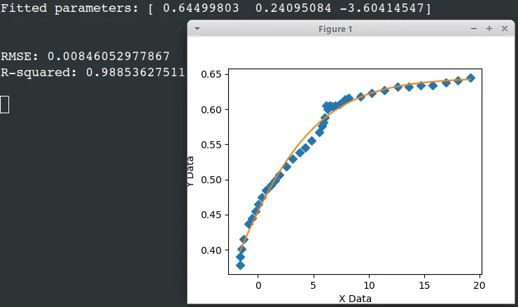
这是一个使用您的方程和振幅缩放因子对我的测试数据进行拟合的示例图形拟合器。此代码使用scipy的差分进化遗传算法为curve_fit()提供初始参数估计,因为scipy默认的所有1.0的初始参数估计并不总是最优的。Differential Evolution的scipy实现使用拉丁超立方体算法来确保对参数空间进行彻底搜索,这需要边界来进行搜索。在这个例子中,这些边界取自我提供的示例数据,当使用自己的数据时,请检查边界是否合理。请注意,与初始参数估计的具体值相比,参数范围要容易得多。
import numpy, scipy, matplotlib
import matplotlib.pyplot as plt
from scipy.optimize import curve_fit
from scipy.optimize import differential_evolution
import warnings
xData = numpy.array([19.1647, 18.0189, 16.9550, 15.7683, 14.7044, 13.6269, 12.6040, 11.4309, 10.2987, 9.23465, 8.18440, 7.89789, 7.62498, 7.36571, 7.01106, 6.71094, 6.46548, 6.27436, 6.16543, 6.05569, 5.91904, 5.78247, 5.53661, 4.85425, 4.29468, 3.74888, 3.16206, 2.58882, 1.93371, 1.52426, 1.14211, 0.719035, 0.377708, 0.0226971, -0.223181, -0.537231, -0.878491, -1.27484, -1.45266, -1.57583, -1.61717])
yData = numpy.array([0.644557, 0.641059, 0.637555, 0.634059, 0.634135, 0.631825, 0.631899, 0.627209, 0.622516, 0.617818, 0.616103, 0.613736, 0.610175, 0.606613, 0.605445, 0.603676, 0.604887, 0.600127, 0.604909, 0.588207, 0.581056, 0.576292, 0.566761, 0.555472, 0.545367, 0.538842, 0.529336, 0.518635, 0.506747, 0.499018, 0.491885, 0.484754, 0.475230, 0.464514, 0.454387, 0.444861, 0.437128, 0.415076, 0.401363, 0.390034, 0.378698])
def sigmoid(x, amplitude, x0, k):
return amplitude * 1.0/(1.0+numpy.exp(-x0*(x-k)))
def sumOfSquaredError(parameterTuple):
warnings.filterwarnings("ignore")
val = sigmoid(xData, *parameterTuple)
return numpy.sum((yData - val) ** 2.0)
def generate_Initial_Parameters():
maxX = max(xData)
minX = min(xData)
maxY = max(yData)
minY = min(yData)
parameterBounds = []
parameterBounds.append([minY, maxY])
parameterBounds.append([minX, maxX])
parameterBounds.append([minX, maxX])
result = differential_evolution(sumOfSquaredError, parameterBounds, seed=3)
return result.x
geneticParameters = generate_Initial_Parameters()
fittedParameters, pcov = curve_fit(sigmoid, xData, yData, geneticParameters)
print('Fitted parameters:', fittedParameters)
print()
modelPredictions = sigmoid(xData, *fittedParameters)
absError = modelPredictions - yData
SE = numpy.square(absError)
MSE = numpy.mean(SE)
RMSE = numpy.sqrt(MSE)
Rsquared = 1.0 - (numpy.var(absError) / numpy.var(yData))
print()
print('RMSE:', RMSE)
print('R-squared:', Rsquared)
print()
def ModelAndScatterPlot(graphWidth, graphHeight):
f = plt.figure(figsize=(graphWidth/100.0, graphHeight/100.0), dpi=100)
axes = f.add_subplot(111)
axes.plot(xData, yData, 'D')
xModel = numpy.linspace(min(xData), max(xData))
yModel = sigmoid(xModel, *fittedParameters)
axes.plot(xModel, yModel)
axes.set_xlabel('X Data')
axes.set_ylabel('Y Data')
plt.show()
plt.close('all')
graphWidth = 800
graphHeight = 600
ModelAndScatterPlot(graphWidth, graphHeight)