在Python中拟合指数增长函数曲线

Question

我有以下数据点需要进行曲线拟合：

import matplotlib.pyplot as plt
import numpy as np
from scipy.optimize import curve_fit

t = np.array([15474.6, 15475.6, 15476.6, 15477.6, 15478.6, 15479.6, 15480.6,
              15481.6, 15482.6, 15483.6, 15484.6, 15485.6, 15486.6, 15487.6,
              15488.6, 15489.6, 15490.6, 15491.6, 15492.6, 15493.6, 15494.6,
              15495.6, 15496.6, 15497.6, 15498.6, 15499.6, 15500.6, 15501.6,
              15502.6, 15503.6, 15504.6, 15505.6, 15506.6, 15507.6, 15508.6,
              15509.6, 15510.6, 15511.6, 15512.6, 15513.6])

v = np.array([4.082, 4.133, 4.136, 4.138, 4.139, 4.14, 4.141, 4.142, 4.143,
              4.144, 4.144, 4.145, 4.145, 4.147, 4.146, 4.147, 4.148, 4.148,
              4.149, 4.149, 4.149, 4.15, 4.15, 4.15, 4.151, 4.151, 4.152,
              4.152, 4.152, 4.153, 4.153, 4.153, 4.153, 4.154, 4.154, 4.154,
              4.154, 4.154, 4.155, 4.155])

我想要拟合到数据的指数函数是：

以下是代表上述公式的Python函数及其与数据相关的曲线拟合的详细信息：

def func(t, a, b, alpha):
    return a - b * np.exp(-alpha * t)


# scale vector to start at zero otherwise exponent is too large
t_scale = t - t[0]

# initial guess for curve fit coefficients
a0 = v[-1]
b0 = v[0]
alpha0 = 1/t_scale[-1]

# coefficients and curve fit for curve
popt4, pcov4 = curve_fit(func, t_scale, v, p0=(a0, b0, alpha0))

a, b, alpha = popt4
v_fit = func(t_scale, a, b, alpha)

ss_res = np.sum((v - v_fit) ** 2)       # residual sum of squares
ss_tot = np.sum((v - np.mean(v)) ** 2)  # total sum of squares
r2 = 1 - (ss_res / ss_tot)              # R squared fit, R^2

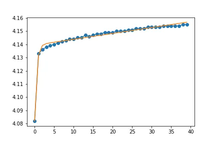
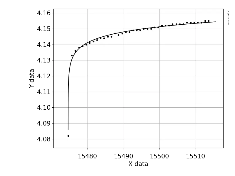
以下是与曲线拟合相比的数据绘图。还提供了参数和R平方值。

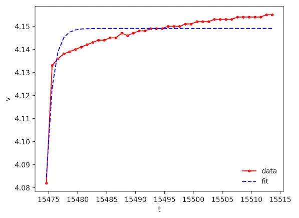
a0 = 4.1550   b0 = 4.0820   alpha0 = 0.0256
a = 4.1490    b = 0.0645    alpha = 0.9246
R² = 0.8473

使用上述方法能否更好地拟合数据，还是需要使用不同形式的指数方程？

我也不确定初始值（a0、b0、alpha0）应该使用什么。在示例中，我选择了数据点，但这可能不是最佳方法。有没有关于曲线拟合系数的初始猜测的建议？

- wigging

---

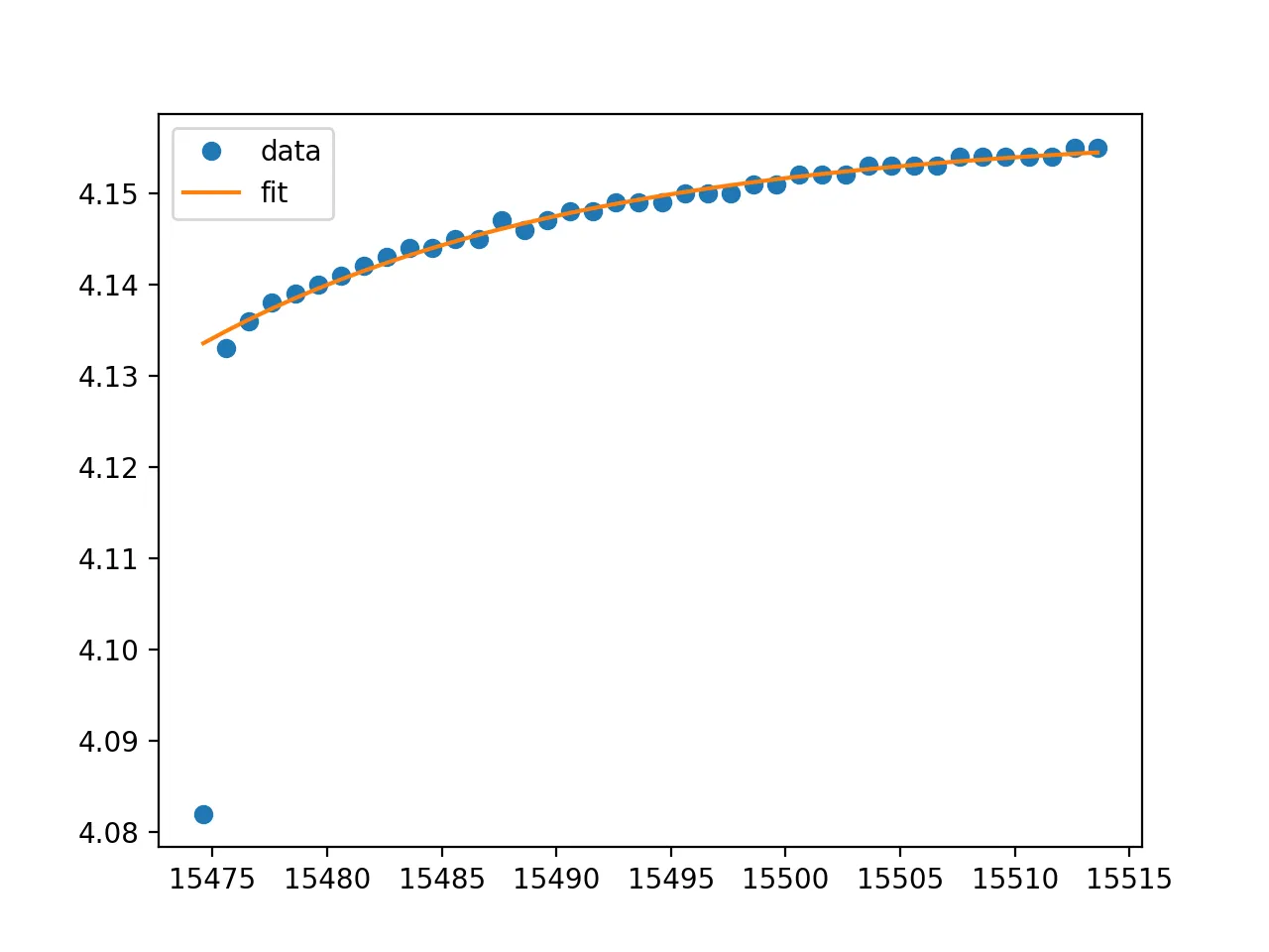
我会尝试两种方法：1. 不要通过峰值，2. 给一些点添加权重，以便将拟合向下拉。您可以使用 curve_fit 的 sigma 参数来实现。 - dan_g

@user3014097 我之前不知道 sigma 这个关键字。我该如何在我的例子中应用它？另外，从峰值开始曲线拟合（t[1:] 和 v[1:]）效果很好，但这会对 popt 值产生多大影响呢？ - wigging

方程图在右侧是平的，而数据显示了明显的向上斜坡。我认为这个方程不会很好地适合数据的那一部分。 - James Phillips

Answer 1

我认为这看起来更适合由多个组件完成，而不是一个单独的指数。

def func(t, a, b, c, d, e):
    return a*np.exp(-t/b) + c*np.exp(-t/d) + e


# scale vector to start at zero otherwise exponent is too large
t_scale = t - t[0]

# initial guess for curve fit coefficients
guess = [1, 1, 1, 1, 0]

# coefficients and curve fit for curve
popt, pcov = curve_fit(func, t_scale, v, p0=guess)

v_fit = func(t_scale, *popt)

- dan_g

---

您使用的方程式提供了更好的拟合效果。然而，解决方案似乎对初始猜测值非常敏感。例如，a、c 和 e 的初始值可以用 v[-1]、v[0] 和 v[-1] 表示。是否有一种不那么敏感于初始值的方法？ - wigging

为了使初始值与我的原始问题类似，看起来你的示例中 a、c 和 e 的初始猜测应该是从 v[-1] 中获取的值。这是否合理？ - wigging

我不确定你最初的问题是什么。想想在t = 0时方程会是什么样子。基本上，它应该是你两个组件的最小值之和加上偏移量（E）。只要你的猜测大致正确，你就应该没问题。通常情况下，当我进行这种拟合时，我更喜欢将时间（你已经做到了）和我的基线都归零（因此，在你的情况下v_scale = v - v.max()），这样你就可以衰减到0。但是，只要你的猜测在合理范围内，你就应该没问题。如果v变化很大，我会在拟合之前对其进行归一化处理。 - dan_g

另一个解决方案是将v转换为线性，这将使拟合步骤更简单。 - dan_g

你是指线性回归，其中你会取方程的对数并拟合到该形式吗？你能提供一个例子吗？感谢您的所有帮助。 - wigging

Answer 2

如果您删除第一个数据点，拟合效果会更好。

使用lmfit（https://lmfit.github.io/lmfit-py），它提供了一个更高级和更易于使用的曲线拟合接口，您的拟合脚本将如下所示：

import matplotlib.pyplot as plt
import numpy as np
from lmfit import Model

t = np.array([15474.6, 15475.6, 15476.6, 15477.6, 15478.6, 15479.6, 15480.6,
              15481.6, 15482.6, 15483.6, 15484.6, 15485.6, 15486.6, 15487.6,
              15488.6, 15489.6, 15490.6, 15491.6, 15492.6, 15493.6, 15494.6,
              15495.6, 15496.6, 15497.6, 15498.6, 15499.6, 15500.6, 15501.6,
              15502.6, 15503.6, 15504.6, 15505.6, 15506.6, 15507.6, 15508.6,
              15509.6, 15510.6, 15511.6, 15512.6, 15513.6])

v = np.array([4.082, 4.133, 4.136, 4.138, 4.139, 4.14, 4.141, 4.142, 4.143,
              4.144, 4.144, 4.145, 4.145, 4.147, 4.146, 4.147, 4.148, 4.148,
              4.149, 4.149, 4.149, 4.15, 4.15, 4.15, 4.151, 4.151, 4.152,
              4.152, 4.152, 4.153, 4.153, 4.153, 4.153, 4.154, 4.154, 4.154,
              4.154, 4.154, 4.155, 4.155])

def func(t, a, b, alpha):
    return a + b * np.exp(-alpha * t)

# remove first data point, take offset from t
tx = t[1:] - t[0]
vx = v[1:]

# turn your model function into a Model
amodel = Model(func)
# create parameters with initial values.  Note that parameters
# are named from the arguments of your model function.
params = amodel.make_params(a=v[0], b=0, alpha=1.0/(t[-1]-t[0]))

# fit the data to the model with the parameters
result = amodel.fit(vx, params, t=tx)

# print the fit statistics and resulting parameters
print(result.fit_report())

# plot data and fit
plt.plot(t, v, 'o', label='data')
plt.plot(t, result.eval(result.params, t=(t-t[0])), '--', label='fit')
plt.legend()
plt.show()

这将打印出这些结果

[[Model]]
    Model(func)
[[Fit Statistics]]
    # fitting method   = leastsq
    # function evals   = 44
    # data points      = 39
    # variables        = 3
    chi-square         = 1.1389e-05
    reduced chi-square = 3.1635e-07
    Akaike info crit   = -580.811568
    Bayesian info crit = -575.820883
[[Variables]]
    a:      4.15668660 +/- 5.0662e-04 (0.01%) (init = 4.082)
    b:     -0.02312772 +/- 4.1930e-04 (1.81%) (init = 0)
    alpha:  0.06004740 +/- 0.00360126 (6.00%) (init = 0.02564103)
[[Correlations]] (unreported correlations are < 0.100)
    C(a, alpha) = -0.945
    C(a, b)     = -0.682
    C(b, alpha) =  0.465

并显示此拟合图：

- M Newville

---

请使用与问题提出者在其问题中使用的相同图形缩放重新绘制，以便进行比较。 - James Phillips

我不明白为什么有人给这个答案点了踩。当我看到问题中的图表时，"删除第一个点"是我首先想到的事情。这个答案让我省去了去找出它是否有效的麻烦——结果表明它效果很好！ - Warren Weckesser

@JamesPhillips 非常好的建议。我更新了图表，包括第一个点。这真正说明了那个点是多么的异常值。 - M Newville

如果第一点和第二点之间有更多的数据，情况可能会有所不同，但这里并非如此。如果可能的话，我建议在这个范围内获取额外的数据。缺少这些额外的数据，你有很强的理由根据回归分析删除那个数据点。感谢更新的图表。 - James Phillips

通过移除初始点，这会对变量a、b和alpha的值产生多大影响？ - wigging

@wigging 对我来说，第一个点看起来像是一个异常值。您可以使用t[:]和v[:]而不是t[1:]和v[1:]来轻松检查包含它的结果。卡方将增加约75倍（拟合程度更差），a约为4.1，b约为-0.064，alpha约为0.92。拟合效果将与您最初的问题一样糟糕。正如其他答案所指出的那样，具有第一个点的数据与您的模型不匹配，他们提出了其他更好的模型。忽略第一个点，您的数据可以匹配您的模型。 - M Newville

Answer 3

我找到的最佳单一3参数方程式是一个x平移的幂函数，R平方=0.9952：

y = pow((a + x), b) + Offset

带参数的：

a = -1.5474599569484271E+04
b =  6.3963649365056151E-03
Offset =  3.1303674911990789E+00

- James Phillips