你好,我正在尝试使用多项式或指数函数拟合我的数据,但两者都失败了。我使用的代码如下:
with open('argon.dat','r') as f:
    argon=f.readlines()

eng1 = np.array([float(argon[argon.index(i)].split('\n')[0].split('  ')[0])*1000 for i in argon])
II01 = np.array([1-math.exp(-float(argon[argon.index(i)].split('\n')[0].split('  ')[1])*(1.784e-3*6.35)) for i in argon])

with open('copper.dat','r') as f:
    copper=f.readlines()

eng2 = [float(copper[copper.index(i)].split('\n')[0].split('  ')[0])*1000 for i in copper]
II02 = [math.exp(-float(copper[copper.index(i)].split('\n')[0].split('  ')[1])*(8.128e-2*8.96)) for i in copper]

fig, ax1 = plt.subplots(figsize=(12,10))
ax2 = ax1.twinx()
ax1.set_yscale('log')
ax2.set_yscale('log')

arg = ax2.plot(eng1, II01, 'b--', label='Argon gas absorption at STP (6.35 cm)')
cop = ax1.plot(eng2, II02, 'r', label='Copper wall transp. (0.81 mm)')
plot = arg+cop

labs = [l.get_label() for l in plot]
ax1.legend(plot,labs,loc='lower right', fontsize=14)
ax1.set_ylim(1e-6,1)
ax2.set_ylim(1e-6,1)
ax1.set_xlim(0,160)
ax1.set_ylabel(r'$\displaystyle I/I_0$', fontsize=18)
ax2.set_ylabel(r'$\displaystyle 1-I/I_0$', fontsize=18)
ax1.set_xlabel('Photon Energy [keV]', fontsize=18)
plt.show()
这让我想起了
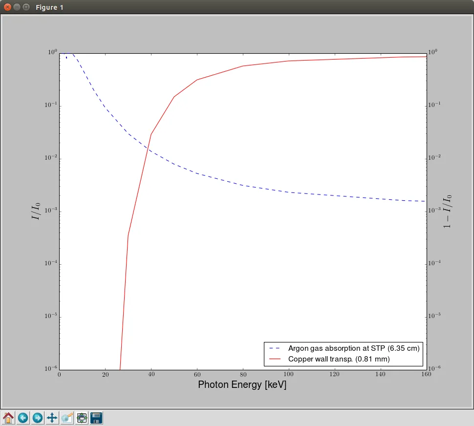 。我的目标是,不再按照这种方式绘制数据,而是将它们适配到指数曲线,并将这些曲线相乘,以得出探测器效率(我试过按元素相乘,但没有足够的数据点来获得平滑的曲线)。我尝试使用polyfit,并尝试定义一个指数函数来检查它是否奏效,然而在两种情况下都得到了一条直线。
#def func(x, a, c, d):
#    return a*np.exp(-c*x)+d
#
#popt, pcov = curve_fit(func, eng1, II01)
#plt.plot(eng1, func(eng1, *popt), label="Fitted Curve")
并且
model = np.polyfit(eng1, II01 ,5)
y = np.poly1d(model)
#splineYs = np.exp(np.polyval(model,eng1)) # also tried this but didnt work
ax2.plot(eng1,y)
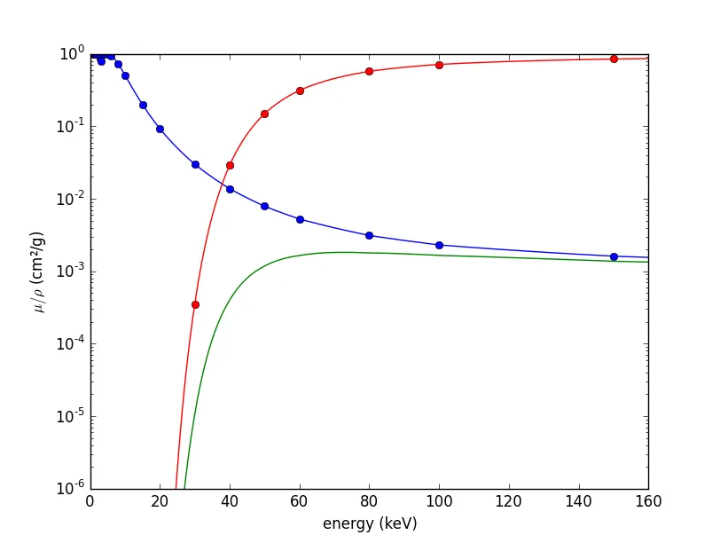
需要时,数据将从http://www.nist.gov/pml/data/xraycoef/index.cfm获取。同样的工作可以在图3中找到:http://scitation.aip.org/content/aapt/journal/ajp/83/8/10.1119/1.4923022 @Oliver回答后,其余部分已经进行了修改:
我通过使用现有数据进行了乘法运算:
i = 0
eff1 = []
while i < len(arg):
    eff1.append(arg[i]*cop[i])
    i += 1
我得到的结果是(红色:铜,虚线蓝色:氩,蓝色:乘法)。
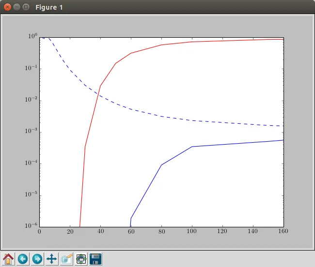 这是我希望得到的结果,但通过使用曲线函数,这将是一个平滑的曲线,而我想最终得到这个结果(在@oliver的答案下已经发表了评论,指出了什么是错误或误解)。
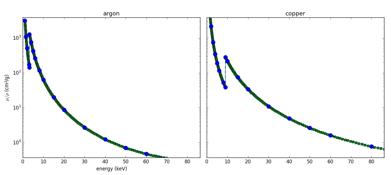
μ/ρ与能量之间的关系是不同的。不过我已经进行了快速编辑,因为我遗漏了new_limits是什么:它基于第二列中的值,而不是第一列。 - Oliver W.