指数曲线拟合无法拟合

Question

尝试将一组数据绘制成指数曲线时：

import matplotlib
import matplotlib.pyplot as plt
from matplotlib import style
from matplotlib import pylab
import numpy as np
from scipy.optimize import curve_fit

x = np.array([30,40,50,60])
y = np.array([0.027679854,0.055639098,0.114814815,0.240740741])

def exponenial_func(x, a, b, c):
    return a*np.exp(-b*x)+c

popt, pcov = curve_fit(exponenial_func, x, y, p0=(1, 1e-6, 1))

xx = np.linspace(10,60,1000)
yy = exponenial_func(xx, *popt)

plt.plot(x,y,'o', xx, yy)
pylab.title('Exponential Fit')
ax = plt.gca()
fig = plt.gcf()

plt.xlabel(r'Temperature, C')
plt.ylabel(r'1/Time, $s^-$$^1$')

plt.show()

上述代码的图表:

然而，当我添加数据点20 (x) 和 0.015162344 (y) 时:

import matplotlib
import matplotlib.pyplot as plt
from matplotlib import style
from matplotlib import pylab
import numpy as np
from scipy.optimize import curve_fit

x = np.array([20,30,40,50,60])
y = np.array([0.015162344,0.027679854,0.055639098,0.114814815,0.240740741])

def exponenial_func(x, a, b, c):
    return a*np.exp(-b*x)+c

popt, pcov = curve_fit(exponenial_func, x, y, p0=(1, 1e-6, 1))

xx = np.linspace(20,60,1000)
yy = exponenial_func(xx, *popt)

plt.plot(x,y,'o', xx, yy)
pylab.title('Exponential Fit')
ax = plt.gca()
fig = plt.gcf()

plt.xlabel(r'Temperature, C')
plt.ylabel(r'1/Time, $s^-$$^1$')

plt.show()

上述代码会生成错误信息：

'RuntimeError: Optimal parameters not found: Number of calls to function has reached maxfev = 800.'

如果将maxfev设置为maxfev = 1300，则会解决该问题。

popt, pcov = curve_fit(exponenial_func, x, y, p0=(1, 1e-6, 1),maxfev=1300)

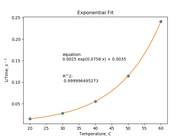
图形绘制出来了，但曲线拟合不正确。通过上述代码更改图形，maxfev = 1300：

我认为这是因为点20和30太靠近了吗？相比之下，Excel将数据绘制为如下：

我该如何正确绘制此曲线？

- gravitypulling

---

将您初始猜测p0=(1,1e-6,0)的最后一个值进行更改，对我来说可以正确拟合数据。 - DavidG

谢谢DavidG，这对我也有效。 - gravitypulling

Answer 1

根据您的数据，很明显您需要一个正指数，因此，在使用 a*np.exp(-b*x) + c 作为基本模型时，b需要是负数。然而，您却以正值作为b的初始值，这很可能导致问题。

如果您将其更改为：

popt, pcov = curve_fit(exponenial_func, x, y, p0=(1, 1e-6, 1))

to

popt, pcov = curve_fit(exponenial_func, x, y, p0=(1, -1e-6, 1))

它很好地运行并给出了预期的结果。

或者，您也可以将方程式更改为

return a*np.exp(b*x) + c

并且从你原先的初始值开始。

这是完整的代码：

import matplotlib.pyplot as plt
import numpy as np
from scipy.optimize import curve_fit


def exponenial_func(x, a, b, c):
    return a*np.exp(b*x)+c


x = np.array([20, 30, 40, 50, 60])
y = np.array([0.015162344, 0.027679854, 0.055639098, 0.114814815, 0.240740741])


popt, pcov = curve_fit(exponenial_func, x, y, p0=(1, 1e-6, 1))

xx = np.linspace(20, 60, 1000)
yy = exponenial_func(xx, *popt)

# please check whether that is correct
r2 = 1. - sum((exponenial_func(x, *popt) - y) ** 2) / sum((y - np.mean(y)) ** 2)

plt.plot(x, y, 'o', xx, yy)
plt.title('Exponential Fit')
plt.xlabel(r'Temperature, C')
plt.ylabel(r'1/Time, $s^-$$^1$')
plt.text(30, 0.15, "equation:\n{:.4f} exp({:.4f} x) + {:.4f}".format(*popt))
plt.text(30, 0.1, "R^2:\n {}".format(r2))

plt.show()

- Cleb

---

谢谢，我该如何添加直线方程和R^2值？ - gravitypulling

@gravitypulling：您想在哪里添加它？在图形本身中吗？ - Cleb

我想把它添加到图表本身中。 - gravitypulling

@gravitypulling：请检查更新后的答案。同时请确认r2计算是否符合您的意图；如果不是，请更改它。由于您相对较新：如果答案解决了您的问题，请接受答案（点击答案旁边的复选框，然后变为绿色）。 - Cleb

非常感谢，这是非常有信息量的解释，而且是正确的。 - gravitypulling