time = 1:100
head(y)
0.07841589 0.07686316 0.07534116 0.07384931 0.07238699 0.07095363
plot(time,y)
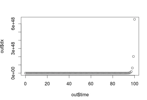
不知道公式,如何在此曲线上拟合一条直线?我无法使用“nls”,因为公式未知(只有数据点)。
如何获得此曲线的方程,并确定方程中的常数?我尝试了loess,但没有给出截距。
time = 1:100
head(y)
0.07841589 0.07686316 0.07534116 0.07384931 0.07238699 0.07095363
plot(time,y)
不知道公式,如何在此曲线上拟合一条直线?我无法使用“nls”,因为公式未知(只有数据点)。
如何获得此曲线的方程,并确定方程中的常数?我尝试了loess,但没有给出截距。
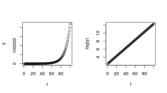
t <- 1:100      # these are your time points
a <- 10         # assume the size at t = 0 is 10
r <- 0.1        # assume a growth constant
y <- a*exp(r*t) # generate some y observations from our exponential model

# visualise
par(mfrow = c(1, 2))
plot(t, y)      # on the original scale
plot(t, log(y)) # taking the log(y)
nls()函数)lm()函数)set.seed(12) # for reproducible results
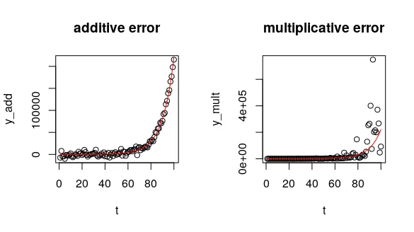
# errors constant across time - additive
y_add <- a*exp(r*t) + rnorm(length(t), sd = 5000) # or: rnorm(length(t), mean = a*exp(r*t), sd = 5000)
# errors grow as y grows - multiplicative (constant on the log-scale)
y_mult <- a*exp(r*t + rnorm(length(t), sd = 1)) # or: rlnorm(length(t), mean = log(a) + r*t, sd = 1)
# visualise
par(mfrow = c(1, 2))
plot(t, y_add, main = "additive error")
lines(t, a*exp(t*r), col = "red")
plot(t, y_mult, main = "multiplicative error")
lines(t, a*exp(t*r), col = "red")
nls(),因为误差在t上是恒定的。使用nls()时,我们需要指定一些优化算法的起始值(尽量“猜测”这些值,因为nls()经常难以收敛到一个解决方案)。add_nls <- nls(y_add ~ a*exp(r*t),
start = list(a = 0.5, r = 0.2))
coef(add_nls)
# a r
# 11.30876845 0.09867135
coef()函数,我们可以获得两个参数的估计值。这给了我们不错的估计值,接近于我们模拟的结果(a = 10和r = 0.1)。plot(t, resid(add_nls))
abline(h = 0, lty = 2)
y_mult 模拟值),我们应该在对数转换后的数据上使用 lm(),因为在该尺度上误差是恒定的。mult_lm <- lm(log(y_mult) ~ t)
coef(mult_lm)
# (Intercept) t
# 2.39448488 0.09837215
(Intercept)相当于我们模型中的log(a),而t是时间变量的系数,等价于我们的r。
要有意义地解释(Intercept),我们可以取它的指数(exp(2.39448488)),得到约10.96,这非常接近我们的模拟值。nls函数拟合误差是乘法的数据,会发生什么:mult_nls <- nls(y_mult ~ a*exp(r*t), start = list(a = 0.5, r = 0.2))
coef(mult_nls)
# a r
# 281.06913343 0.06955642
# get the model's coefficients
lm_coef <- coef(mult_lm)
nls_coef <- coef(mult_nls)

# make the plot
plot(t, y_mult)
lines(t, a*exp(r*t), col = "brown", lwd = 5)
lines(t, exp(lm_coef[1])*exp(lm_coef[2]*t), col = "dodgerblue", lwd = 2)
lines(t, nls_coef[1]*exp(nls_coef[2]*t), col = "orange2", lwd = 2)
legend("topleft", col = c("brown", "dodgerblue", "orange2"),
       legend = c("known model", "nls fit", "lm fit"), lwd = 3)
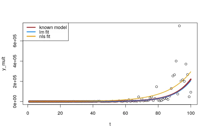
lm() 拟合要比对原始数据使用 nls() 拟合好得多。plot(t, resid(mult_nls))
abline(h = 0, lty = 2)
lm()或nls(),这里有一个很好的讨论https://stats.stackexchange.com/questions/61747/linear-vs-nonlinear-regression?rq=1 - Alejo Bernardinlm)与拟合非线性模型(使用nls)得到的结果不同,因为最小化的距离不同。对于对数化的线性模型,对数化的残差被最小化,从而产生了偏差,使得剩余较大的残差偏离。因此,增长的开始更容易被错误地估计。 - Mario Reutter很遗憾,取对数并拟合线性模型不是最优解。原因是,当将指数函数应用于返回原始模型时,大y值的误差的权重要比小y值的误差更大。以下是一个例子:
f <- function(x){exp(0.3*x+5)}

squaredError <- function(a,b,x,y) {sum((exp(a*x+b)-f(x))^2)}

x <- 0:12
y <- f(x) * ( 1 + sample(-300:300,length(x),replace=TRUE)/10000 )
x
y
#--------------------------------------------------------------------

M <- lm(log(y)~x)
a <- unlist(M[1])[2]
b <- unlist(M[1])[1]
print(c(a,b))

squaredError(a,b,x,y)

approxPartAbl_a <- (squaredError(a+1e-8,b,x,y) - squaredError(a,b,x,y))/1e-8

for ( i in 0:10 )
{
  eps <- -i*sign(approxPartAbl_a)*1e-5
  print(c(eps,squaredError(a+eps,b,x,y)))
}
结果:
> f <- function(x){exp(0.3*x+5)}

> squaredError <- function(a,b,x,y) {sum((exp(a*x+b)-f(x))^2)}

> x <- 0:12

> y <- f(x) * ( 1 + sample(-300:300,length(x),replace=TRUE)/10000 )

> x
 [1]  0  1  2  3  4  5  6  7  8  9 10 11 12

> y
 [1]  151.2182  203.4020  278.3769  366.8992  503.5895  682.4353  880.1597 1186.5158 1630.9129 2238.1607 3035.8076 4094.6925 5559.3036

> #--------------------------------------------------------------------
>
> M <- lm(log(y)~x)

> a <- unlist(M[1])[2]

> b <- unlist(M[1])[1]

> print(c(a,b))
          coefficients.x coefficients.(Intercept)
               0.2995808                5.0135529

> squaredError(a,b,x,y)
[1] 5409.752

> approxPartAbl_a <- (squaredError(a+1e-8,b,x,y) - squaredError(a,b,x,y))/1e-8

> for ( i in 0:10 )
+ {
+   eps <- -i*sign(approxPartAbl_a)*1e-5
+   print(c(eps,squaredError(a+eps,b,x,y)))
+ }
[1]    0.000 5409.752
[1]   -0.00001 5282.91927
[1]   -0.00002 5157.68422
[1]   -0.00003 5034.04589
[1]   -0.00004 4912.00375
[1]   -0.00005 4791.55728
[1]   -0.00006 4672.70592
[1]   -0.00007 4555.44917
[1]   -0.00008 4439.78647
[1]   -0.00009 4325.71730
[1]   -0.0001 4213.2411
>
也许可以尝试一些数值方法,比如梯度搜索,来找到平方误差函数的最小值。
如果确实是指数关系,你可以尝试取对数,并将线性模型拟合到这个变量上。