很想看看你的数据集。
无论如何,这是一个可行的例子。希望能对你有所帮助。
logfit <- function(x,jpw) {
   jpw[1] + jpw[2]/(1+exp(-((x-jpw[3])/jpw[4])))
}

jpw <- c(-2,1,0,.5)
x <- runif(100, -3, 3)
y <- logfit(x, jpw)+rnorm(100, sd=0.01)
df <- data.frame(x,y)

curve(logfit(x,jpw),from=-3,to=3, ,type='l')
points(x,y)
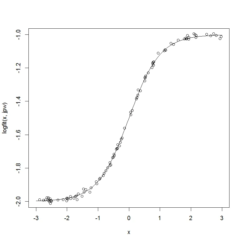
fitmodel <- nls(y ~ a + b/(1+exp(-((x-c)/d))),
    data = df,
    start=list(a=1, b=2, c=1, d=1),
    trace=TRUE)

fitmodel
输出结果为:
Nonlinear regression model
  model: y ~ a + b/(1 + exp(-((x - c)/d)))
   data: df
        a         b         c         d
-1.999901  1.002425  0.006527  0.498689
 residual sum-of-squares: 0.009408

Number of iterations to convergence: 6
Achieved convergence tolerance: 1.732e-06
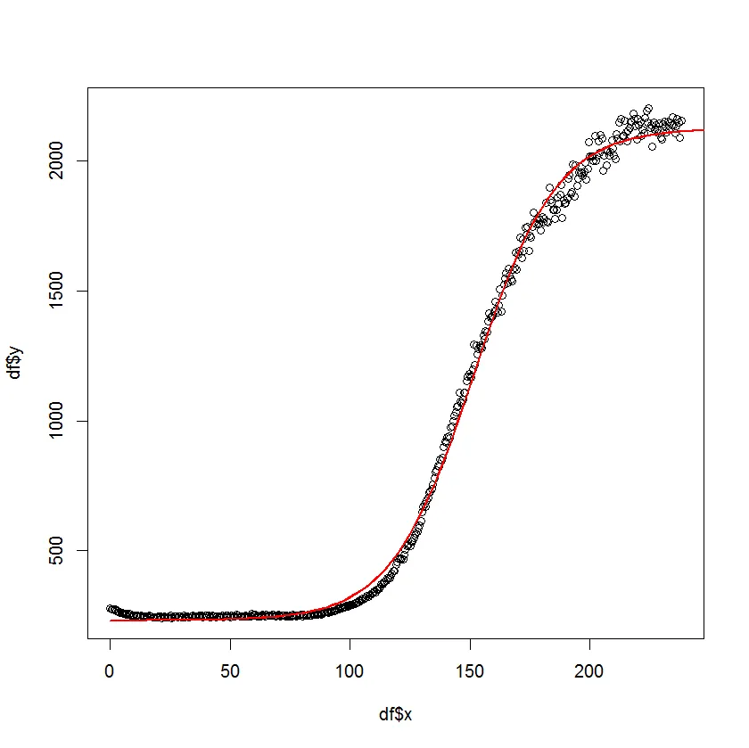
这里我使用@jpw提供的数据。
df <- dget(file="data.txt")
names(df) <- c("y","v2","x")
fitmodel <- nls(y ~ a + b/(1+exp(-((x-c)/d))),
    data = df,
    start=list(a=200,b=2000, c=80, d=10.99),
    trace=TRUE)
summary(fitmodel)
估计的参数为:
Formula: y ~ a + b/(1 + exp(-((x - c)/d)))

Parameters:
   Estimate Std. Error t value Pr(>|t|)
a  231.6587     2.8498   81.29   <2e-16 ***
b 1893.0646     6.3528  297.99   <2e-16 ***
c  151.5405     0.2016  751.71   <2e-16 ***
d   17.2068     0.1779   96.72   <2e-16 ***
---
Signif. codes:  0 ‘***’ 0.001 ‘**’ 0.01 ‘*’ 0.05 ‘.’ 0.1 ‘ ’ 1

Residual standard error: 37.19 on 473 degrees of freedom

Number of iterations to convergence: 10
Achieved convergence tolerance: 3.9e-06
现在我绘制结果。
plot(df$x, df$y)
jpw.est <- coef(fitmodel)
curve(logfit(x,jpw.est), from=0, to=300, col="red", lwd=2, add=T)
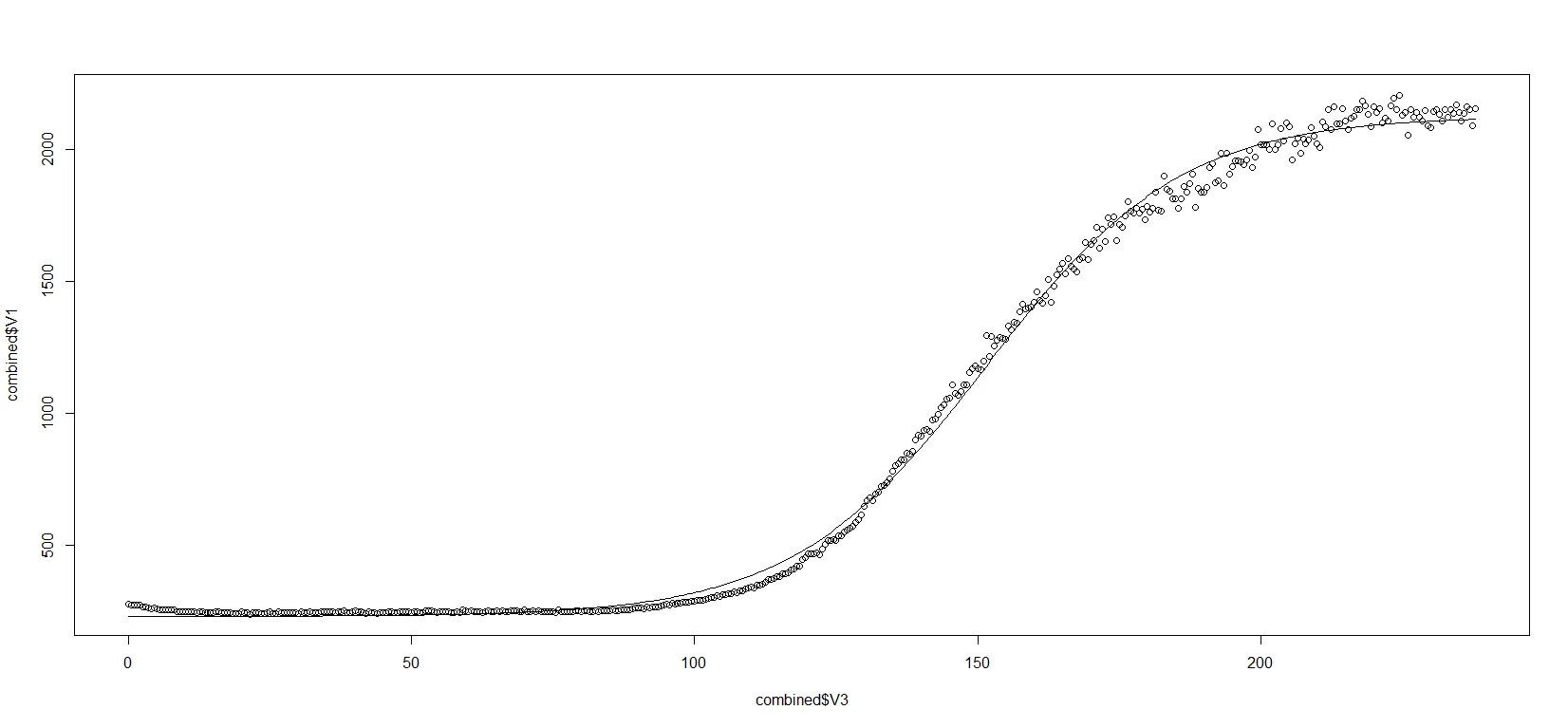
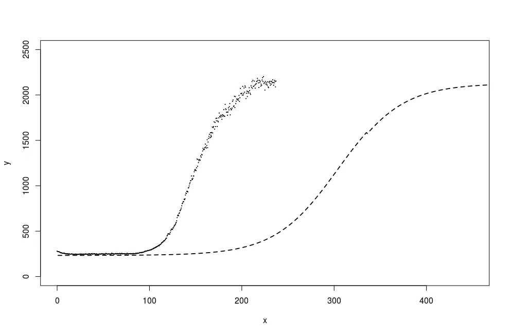
combined有关的问题。它是否包含数字变量x和y? - Andrew Gustary <- mM1$V1 x <- mM1$V3数据看起来像这样: V1 V2 V3 测量值 样本 小时(从0到238,每0.5个小时)我在上面的原始帖子中包含了一张屏幕截图。 - jpw