MATLAB曲线拟合,指数与线性

7

我有一个数据数组,当绘制时看起来像这样。
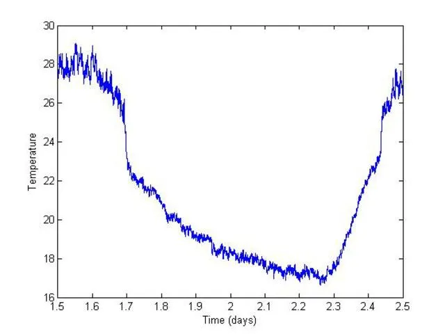
http://s12.postimg.org/7ja47a6b1/temp.jpg

我需要使用 polyfit 命令来确定大致在 1.72.3 之间的时间段内最佳拟合指数。我还必须将此 指数 拟合与简单的 线性 拟合进行比较。

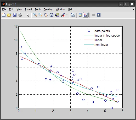
给定方程式为 Temp(t) = Temp0 * exp(-(t-t0)/tau),其中 t0 是对应于温度 Temp0 的时间(我可以选择开始曲线拟合的位置,但必须限制在大约 1.7 和 2.3 之间的区域)。这是我的尝试。

% Arbitrarily defined starting point
t0 = 1.71;

%Exponential fit
p = polyfit(time, log(Temp), 1)
tau = -1./p(1)
Temp0 = exp(p(2))

tm = 1.8:0.01:2.3;
Temp_t = Temp0*exp(-(tm)/tau);
plot(time, Temp, tm, Temp_t)

figure(2)

%Linear fit
p2 = polyfit(time, Temp, 1);
Temp_p = p2(1)*tm + p2(2);
plot(time, Temp, tm, Temp_p)
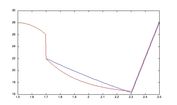
我的指数拟合结果看起来像这样 exponential fit。我的线性拟合看起来像这样 linear fit
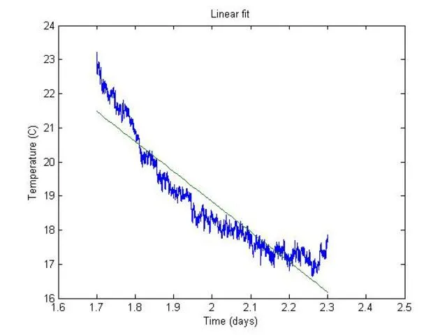
。(几乎相同)。我做错了什么?这两个拟合应该如此相似吗?有人告诉我可能需要使用circshift函数来帮助解决,但我在阅读帮助文件后无法理解该命令的适用性。

@Amro 的链接似乎已被 MathWorks 破坏。更新版本在这里 - horchler
1
感谢@horchler,这是我之前提到的示例的更新链接:通过转换为线性拟合非线性模型的陷阱 - Amro
4个回答

4

正如我在评论中提到的那样,在对数空间中拟合线性模型与拟合非线性模型(两者都是最小二乘意义下)之间存在差异。

统计工具箱中有一个很好的演示,解释了这种情况。下面是代码:

%# sample data
x = [5.72 4.22 5.72 3.59 5.04 2.66 5.02 3.11 0.13 2.26 ...
     5.39 2.57 1.20 1.82 3.23 5.46 3.15 1.84 0.21 4.29 ...
     4.61 0.36 3.76 1.59 1.87 3.14 2.45 5.36 3.44 3.41]';
y = [2.66 2.91 0.94 4.28 1.76 4.08 1.11 4.33 8.94 5.25 ...
     0.02 3.88 6.43 4.08 4.90 1.33 3.63 5.49 7.23 0.88 ...
     3.08 8.12 1.22 4.24 6.21 5.48 4.89 2.30 4.13 2.17]';

xx = linspace(min(x), max(x), 100);

%# linear regression in log-space
%#           y = p2 * exp(p1*x)
%#   => log(y) = log(p2) + p1*x
p_exp = polyfit(x, log(y), 1);
yy1 = exp(p_exp(2)) .* exp(xx .* p_exp(1));

%# linear regression
p_lin = polyfit(x, y, 1);
yy2 = polyval(p_lin, xx);

%# non-linear regression (using previous result as initial coeff)
f = @(p,x) p(2)*exp(p(1)*x);
p_nonlin = nlinfit(x, y, f, [p_exp(1) exp(p_exp(2))]);
yy3 = f(p_nonlin, xx);

plot(x,y,'o', xx,yy1,'-', xx,yy2,'-', xx,yy3,'-')
legend({'data points','linear in log-space','linear','non-linear'})

regression


4
事情正在按照您的预期发展。问题在于,您尝试拟合的函数不是数据的很好近似。通过观察曲线,似乎指数部分趋向于一个约为16的值;但是,您使用的函数最终会趋向于0度温度。因此,对22到16范围内的一部分进行拟合将给您一个几乎线性的关系。为了说明这一点,我编写了几行代码,大致匹配了您拥有的数据点,并显示了不同的函数(一个趋向于0,另一个趋向于16)将为您提供非常不同的曲线形状。第一个(原始函数)在22和16之间的T值几乎是线性的 - 因此它看起来像线性拟合。
我建议您考虑“正确”的函数形状 - 是什么基础物理使您选择特定的形式? 这很重要...
以下是代码:
time = linspace(1.5, 2.5, 200);
t0 = 1.7;
t1 = 2.3;
tau = 2.0;

% define three sections of the function:
s1 = find(time < t0);
s2 = find(time >= t0 & time < t1);
s3 = find(time > 2.3);

% compute a shape for the function in each section:
tData(s1) = 28 - 50*(time(s1)-1.5).^2;
tData(s2) = 22*exp(-(time(s2)-t0)/tau);
tData(s3) = tData(s2(end)) + (s3 - s3(1))*12 / numel(s3);

figure
plot(time, tData)

% modify the equation slightly: assume equilibrium temperature is 16
% with a bit of effort one could fit for this as a second parameter
Teq = 16;
tData2 = tData;
tau2 = tau / 8; % decay more strongly to get down to approx the same value by t1
tData2(s2) = (22 - Teq) * exp( - (time(s2) - t0) / tau2) + Teq;
tData2(s3) = tData2(s2(end)) + (s3 - s3(1))*12 / numel(s3);

hold on;
plot(time, tData2, 'r')

这导致产生以下图表:

enter image description here

我从中得出结论,你的图表看起来非常相似的主要原因是你尝试拟合的函数在你选择的域上几乎是线性的 - 不同的函数选择将更好地匹配。

1
非常感谢您,Floris。我很感激您的回复。我被告知要比较两种曲线拟合形式,并确定哪一种更好地拟合了数据。我原以为这些形式会更加明显,但当它们并不明显时,我开始怀疑我的代码。您的答案非常清晰和有用,我非常感谢。 - scimaks

2

如果我理解正确,您在polyfit中使用的time和Temp变量包含所有值(从1.5到2.5)。因此,在计算polyfit之前,您可能希望将time和Temp的值限制在1.71到2.3之间(现在它正在从1.5到2.5计算polyfit,因此该线与数据点不对齐)。

p = polyfit(time, log(Temp), 1)

你说得对,m_power!谢谢。我已经上传了新的拟合数据。指数拟合和线性拟合看起来应该这么相似吗?再次感谢! - scimaks

0

使用

polyfit(x,y,n)

Matlab曲线拟合工具箱中的函数。


网页内容由stack overflow 提供, 点击上面的
可以查看英文原文,
原文链接