从UnivariateSpline对象获取样条方程

Question

从UnivariateSpline对象获取样条方程

12

我正在使用UnivariateSpline来构造我的一些数据的分段多项式。然后我想在其他程序中（无论是C还是FORTRAN）使用这些样条曲线，因此我想了解生成的样条曲线背后的方程。

以下是我的代码：

import numpy as np
import scipy as sp
from  scipy.interpolate import UnivariateSpline
import matplotlib.pyplot as plt
import bisect

data = np.loadtxt('test_C12H26.dat')
Tmid = 800.0
print "Tmid", Tmid
nmid = bisect.bisect(data[:,0],Tmid)
fig = plt.figure()
plt.plot(data[:,0], data[:,7],ls='',marker='o',markevery=20)
npts = len(data[:,0])
#print "npts", npts
w = np.ones(npts)
w[0] = 100
w[nmid] = 100
w[npts-1] = 100
spline1 = UnivariateSpline(data[:nmid,0],data[:nmid,7],s=1,w=w[:nmid])
coeffs = spline1.get_coeffs()
print coeffs
print spline1.get_knots()
print spline1.get_residual()
print coeffs[0] + coeffs[1] * (data[0,0] - data[0,0]) \
                + coeffs[2] * (data[0,0] - data[0,0])**2 \
                + coeffs[3] * (data[0,0] - data[0,0])**3, \
      data[0,7]
print coeffs[0] + coeffs[1] * (data[nmid,0] - data[0,0]) \
                + coeffs[2] * (data[nmid,0] - data[0,0])**2 \
                + coeffs[3] * (data[nmid,0] - data[0,0])**3, \
      data[nmid,7]

print Tmid,data[-1,0]
spline2 = UnivariateSpline(data[nmid-1:,0],data[nmid-1:,7],s=1,w=w[nmid-1:])
print spline2.get_coeffs()
print spline2.get_knots()
print spline2.get_residual()
plt.plot(data[:,0],spline1(data[:,0]))
plt.plot(data[:,0],spline2(data[:,0]))
plt.savefig('test.png')

splines

下面是生成的图表。我相信我在每个间隔中都有有效的样条曲线，但看起来我的样条方程不正确......我在scipy文档中找不到任何相关参考。有人知道吗？谢谢！

- FrenchKheldar

2个回答

2

get_coeffs函数返回的系数是B样条（基样条）系数，这里有详细描述：B-spline (Wikipedia) 很可能你使用的其他程序/语言已经有了实现。只需提供结节位置和系数即可完成设置。

- askewchan

网页内容由stack overflow 提供, 点击上面的

可以查看英文原文，
原文链接

- nzh · Accepted Answer

在 scipy文档中没有提到如何手动生成样条曲线的系数。然而，可以从现有的B样条文献中找到相关内容。以下函数bspleval展示了如何构建B样条基函数（代码中的矩阵B），通过将系数与最高阶基函数相乘并求和，可以轻松地生成样条曲线：

def bspleval(x, knots, coeffs, order, debug=False):
    '''
    Evaluate a B-spline at a set of points.

    Parameters
    ----------
    x : list or ndarray
        The set of points at which to evaluate the spline.
    knots : list or ndarray
        The set of knots used to define the spline.
    coeffs : list of ndarray
        The set of spline coefficients.
    order : int
        The order of the spline.

    Returns
    -------
    y : ndarray
        The value of the spline at each point in x.
    '''

    k = order
    t = knots
    m = alen(t)
    npts = alen(x)
    B = zeros((m-1,k+1,npts))

    if debug:
        print('k=%i, m=%i, npts=%i' % (k, m, npts))
        print('t=', t)
        print('coeffs=', coeffs)

    ## Create the zero-order B-spline basis functions.
    for i in range(m-1):
        B[i,0,:] = float64(logical_and(x >= t[i], x < t[i+1]))

    if (k == 0):
        B[m-2,0,-1] = 1.0

    ## Next iteratively define the higher-order basis functions, working from lower order to higher.
    for j in range(1,k+1):
        for i in range(m-j-1):
            if (t[i+j] - t[i] == 0.0):
                first_term = 0.0
            else:
                first_term = ((x - t[i]) / (t[i+j] - t[i])) * B[i,j-1,:]

            if (t[i+j+1] - t[i+1] == 0.0):
                second_term = 0.0
            else:
                second_term = ((t[i+j+1] - x) / (t[i+j+1] - t[i+1])) * B[i+1,j-1,:]

            B[i,j,:] = first_term + second_term
        B[m-j-2,j,-1] = 1.0

    if debug:
        plt.figure()
        for i in range(m-1):
            plt.plot(x, B[i,k,:])
        plt.title('B-spline basis functions')

    ## Evaluate the spline by multiplying the coefficients with the highest-order basis functions.
    y = zeros(npts)
    for i in range(m-k-1):
        y += coeffs[i] * B[i,k,:]

    if debug:
        plt.figure()
        plt.plot(x, y)
        plt.title('spline curve')
        plt.show()

    return(y)

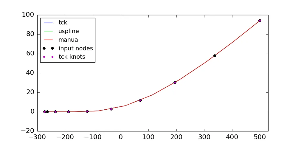
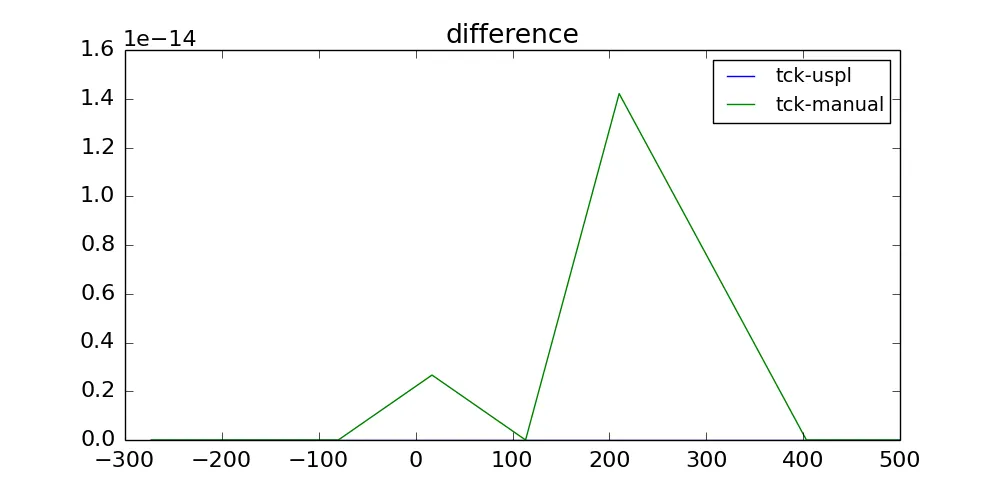
为了举例说明如何将此方法与Scipy现有的单变量样条函数结合使用，以下是一个示例脚本。它采用输入数据并使用Scipy的函数和面向对象的方法进行样条拟合。从这两个方法中获取系数和结点，并将其作为输入传递给我们手动计算的bspleval程序，我们可以复制它们生成的相同曲线。请注意，手动评估曲线和Scipy评估方法之间的差异非常小，几乎肯定是浮点噪声。

x = array([-273.0, -176.4, -79.8, 16.9, 113.5, 210.1, 306.8, 403.4, 500.0])
y = array([2.25927498e-53, 2.56028619e-03, 8.64512988e-01, 6.27456769e+00, 1.73894734e+01,
        3.29052124e+01, 5.14612316e+01, 7.20531200e+01, 9.40718450e+01])

x_nodes = array([-273.0, -263.5, -234.8, -187.1, -120.3, -34.4, 70.6, 194.6, 337.8, 500.0])
y_nodes = array([2.25927498e-53, 3.83520726e-46, 8.46685318e-11, 6.10568083e-04, 1.82380809e-01,
                2.66344008e+00, 1.18164677e+01, 3.01811501e+01, 5.78812583e+01, 9.40718450e+01])

## Now get scipy's spline fit.
k = 3
tck = splrep(x_nodes, y_nodes, k=k, s=0)
knots = tck[0]
coeffs = tck[1]
print('knot points=', knots)
print('coefficients=', coeffs)

## Now try scipy's object-oriented version. The result is exactly the same as "tck": the knots are the
## same and the coeffs are the same, they are just queried in a different way.
uspline = UnivariateSpline(x_nodes, y_nodes, s=0)
uspline_knots = uspline.get_knots()
uspline_coeffs = uspline.get_coeffs()

## Here are scipy's native spline evaluation methods. Again, "ytck" and "y_uspline" are exactly equal.
ytck = splev(x, tck)
y_uspline = uspline(x)
y_knots = uspline(knots)

## Now let's try our manually-calculated evaluation function.
y_eval = bspleval(x, knots, coeffs, k, debug=False)

plt.plot(x, ytck, label='tck')
plt.plot(x, y_uspline, label='uspline')
plt.plot(x, y_eval, label='manual')

## Next plot the knots and nodes.
plt.plot(x_nodes, y_nodes, 'ko', markersize=7, label='input nodes')            ## nodes
plt.plot(knots, y_knots, 'mo', markersize=5, label='tck knots')    ## knots
plt.xlim((-300.0,530.0))
plt.legend(loc='best', prop={'size':14})

plt.figure()
plt.title('difference')
plt.plot(x, ytck-y_uspline, label='tck-uspl')
plt.plot(x, ytck-y_eval, label='tck-manual')
plt.legend(loc='best', prop={'size':14})

plt.show()

enter image description here