Python interp1d与UnivariateSpline的比较

15

我试图将一些MatLab代码移植到Scipy,我尝试了scipy.interpolate中的两个不同函数,interp1dUnivariateSpline。 interp1d的结果与MatLab函数的结果相符,但UnivariateSpline的数字结果不同,而且在某些情况下差别很大。

f = interp1d(row1,row2,kind='cubic',bounds_error=False,fill_value=numpy.max(row2))
return  f(interp)

f = UnivariateSpline(row1,row2,k=3,s=0)
return f(interp)

有人能提供任何见解吗?我的x值并不是等间距的,尽管我不确定为什么会有影响。

4个回答

19

我刚遇到了相同的问题。

简短回答

使用 InterpolatedUnivariateSpline 代替:

f = InterpolatedUnivariateSpline(row1, row2)
return f(interp)

长回答

UnivariateSpline是一种“对给定数据点进行一维平滑样条拟合”的方法,而InterpolatedUnivariateSpline是一种“给定数据点的一维插值样条”。前者平滑数据,而后者则是一种更传统的插值方法,并且产生了与interp1d期望的结果相同。下图说明了它们之间的区别。
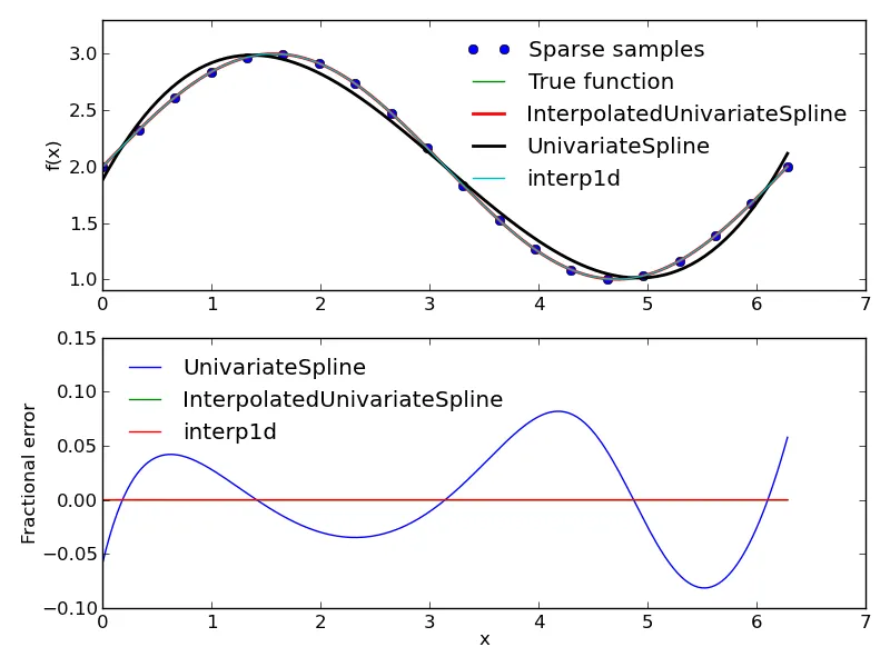
Comparison of interpolation functions

以下是复制该图像所需的代码。

import scipy.interpolate as ip

#Define independent variable
sparse = linspace(0, 2 * pi, num = 20)
dense = linspace(0, 2 * pi, num = 200)

#Define function and calculate dependent variable
f = lambda x: sin(x) + 2
fsparse = f(sparse)
fdense = f(dense)

ax = subplot(2, 1, 1)

#Plot the sparse samples and the true function
plot(sparse, fsparse, label = 'Sparse samples', linestyle = 'None', marker = 'o')
plot(dense, fdense, label = 'True function')

#Plot the different interpolation results
interpolate = ip.InterpolatedUnivariateSpline(sparse, fsparse)
plot(dense, interpolate(dense), label = 'InterpolatedUnivariateSpline', linewidth = 2)

smoothing = ip.UnivariateSpline(sparse, fsparse)
plot(dense, smoothing(dense), label = 'UnivariateSpline', color = 'k', linewidth = 2)

ip1d = ip.interp1d(sparse, fsparse, kind = 'cubic')
plot(dense, ip1d(dense), label = 'interp1d')

ylim(.9, 3.3)

legend(loc = 'upper right', frameon = False)

ylabel('f(x)')

#Plot the fractional error
subplot(2, 1, 2, sharex = ax)

plot(dense, smoothing(dense) / fdense - 1, label = 'UnivariateSpline')
plot(dense, interpolate(dense) / fdense - 1, label = 'InterpolatedUnivariateSpline')
plot(dense, ip1d(dense) / fdense - 1, label = 'interp1d')

ylabel('Fractional error')
xlabel('x')
ylim(-.1,.15)

legend(loc = 'upper left', frameon = False)

tight_layout()

5
这份文档指出InterpolatedUnivariateSpline与s=0的UnivariateSpline等效,而他所使用的正是后者。 - Craig

16
两种方法得出的结果略有不同(但都可能是正确的),原因在于 UnivariateSplineinterp1d 使用的插值方法不同。
  • interp1d 利用您提供给它的 x 值点构造一个平滑的 B 样条曲线。

  • UnivariateSpline 基于 FITPACK,也构造了一个平滑的 B 样条曲线。但是,FITPACK 会尝试选择新的节点以更好地拟合数据(可能是为了最小化 chi^2 加上一些曲率惩罚或类似的东西)。你可以通过 g.get_knots() 查找所使用的节点。

因此,你得到不同结果的原因是插值算法不同。如果你想要基于数据点产生节约,就使用 interp1dsplmake。如果你想要 FITPACK 所做的事情,请使用 UnivariateSpline。在密集数据的极限下,两种方法都会给出相同的结果,但当数据稀疏时,你可能会得到不同的结果。
(我是怎么知道这些的:我阅读了代码 :-)

LSQUnivariateSpline允许您指定节点,因此您可以将它们指定为等于输入?但似乎仍然无法产生相同的输出。 - endolith

2

对我来说没问题。

from scipy import allclose, linspace
from scipy.interpolate import interp1d, UnivariateSpline

from numpy.random import normal

from pylab import plot, show

n = 2**5

x = linspace(0,3,n)
y = (2*x**2 + 3*x + 1) + normal(0.0,2.0,n)

i = interp1d(x,y,kind=3)
u = UnivariateSpline(x,y,k=3,s=0)

m = 2**4

t = linspace(1,2,m)

plot(x,y,'r,')
plot(t,i(t),'b')
plot(t,u(t),'g')

print allclose(i(t),u(t)) # evaluates to True

show()

这给了我一个,

enter image description here


我刚刚运行了以下代码:`from pylab import *` `from scipy.interpolate import *` `x=[3,5,6,8,10]` `y=sin(x)` `z=r_[3:4:.1]` `f=interp1d(x,y,kind=3)` `f1=f(z)` `g=UnivariateSpline(x,y,k=3,s=0)` `g1=g(z)` `print f1-g1`它返回的结果是:[ 1.13797860e-15 -2.14227085e-03 -3.88345765e-03 -5.25282403e-03 -6.27963364e-03 -6.99315013e-03 -7.42263713e-03 -7.59735830e-03 -7.54657727e-03 -7.29955769e-03] - Timothy Dees
@Timothy Dees:啊,我明白问题了。记住,插值是一种用其他函数来近似一个函数的过程;随着你从原始函数中采样更多的点,收敛应该会改善。尝试使用更多的x点来运行你的示例。如果我在大约2 ** 6个点附近进行采样,你的示例对我有效。linspace()使得生成均匀间隔的样本变得容易。 - lafras

0
UnivariateSpline: FITPACK例程的较新封装器。 这可能解释了略有不同的值?(我也发现UnivariateSpline比interp1d快得多。)

它绝对比较快,这也是我想使用它的原因,但它给出的数字与MatLab非常不同,所以我被迫使用更慢的interp1d函数。 - Timothy Dees

网页内容由stack overflow 提供, 点击上面的
可以查看英文原文,
原文链接