使用SciPy进行数值解ODE问题

Question

我在应用 scipy.integrate.odeint 解决下面这个非常简单的ODE时遇到了困难：

y(t)/dt = y(t) + t^2 and y(0) = 0

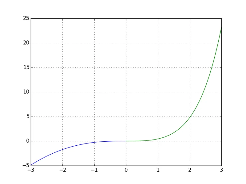
由SciPy计算的解决方案不正确（很可能是因为我在这里混淆了什么），特别是该解决方案未满足初始条件。

import numpy as np
import scipy.integrate
import matplotlib.pyplot as plt
import math

# the definition of the ODE equation
def f(y,t): 
    return [t**2 + y[0]]

# computing the solution
ts = np.linspace(-3,3,1000)
res = scipy.integrate.odeint(f, [0], ts)

# the solution computed by WolframAlpha [1]
def y(t):
    return -t**2 - 2*t + 2*math.exp(t) - 2

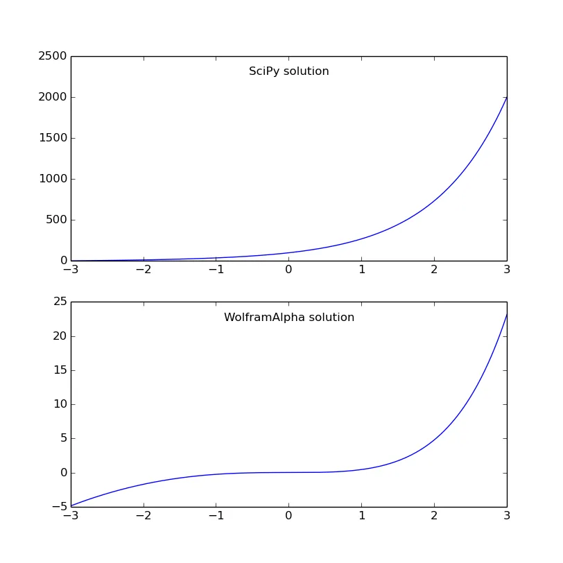
fig = plt.figure(1, figsize=(8,8))

ax1 = fig.add_subplot(211)
ax1.plot(ts, res[:,0])
ax1.text(0.5, 0.95,'SciPy solution', ha='center', va='top',
         transform = ax1.transAxes)

ax1 = fig.add_subplot(212)
ax1.plot(ts, np.vectorize(y)(ts))
ax1.text(0.5, 0.95,'WolframAlpha solution', ha='center', va='top',
         transform = ax1.transAxes)

plt.show()

1 : WolframAlpha: "求解 dy(t)/dt = t^2 + y(t), y(0) = 0"

我的 bug 在哪儿？

- Raffael

Answer 1

您的scipy代码解决了具有初始条件的微分方程，而不是。 odeint的y0参数是在t参数中给出的第一个时间处的值。

要在区间[-3,3]上解决y(0)=0的问题，一种方法是调用两次odeint，如下所示：

In [81]: from scipy.integrate import  odeint

In [82]: def f(y,t): 
   ....:         return [t**2 + y[0]]
   ....: 

In [83]: tneg = np.linspace(0, -3, 500)

In [84]: tpos = np.linspace(0, 3, 500)

In [85]: sol_neg = odeint(f, [0], tneg)

In [86]: sol_pos = odeint(f, [0], tpos)

In [87]: plot(tneg, sol_neg)
Out[87]: [<matplotlib.lines.Line2D at 0x10f890d90>]

In [88]: plot(tpos, sol_pos)
Out[88]: [<matplotlib.lines.Line2D at 0x107a43cd0>]

In [89]: grid(True)

这将创建一个

- Warren Weckesser

---

最简单的解决方案是如何使y（0）= 0，但仍然计算[-3,3]？ - Raffael

也许可以从0计算到3，然后再从0计算到-3。 - Moritz