3D 绘图：在 x 轴上绘制平滑曲线

Question

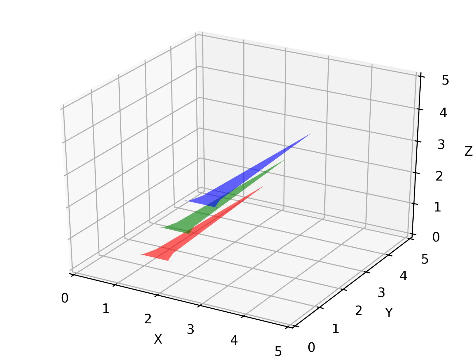
我有一个三维多边形图，想在y轴上平滑该图（即希望它看起来像表面图的切片）。

考虑以下 MWE（摘自此处）：

from mpl_toolkits.mplot3d import Axes3D
from matplotlib.collections import PolyCollection
import matplotlib.pyplot as plt
from matplotlib import colors as mcolors
import numpy as np
from scipy.stats import norm

fig = plt.figure()
ax = fig.gca(projection='3d')

xs = np.arange(-10, 10, 2)
verts = []
zs = [0.0, 1.0, 2.0, 3.0]

for z in zs:
    ys = np.random.rand(len(xs))
    ys[0], ys[-1] = 0, 0
    verts.append(list(zip(xs, ys)))

poly = PolyCollection(verts, facecolors=[mcolors.to_rgba('r', alpha=0.6),
                                         mcolors.to_rgba('g', alpha=0.6), 
                                         mcolors.to_rgba('b', alpha=0.6), 
                                         mcolors.to_rgba('y', alpha=0.6)])
poly.set_alpha(0.7)
ax.add_collection3d(poly, zs=zs, zdir='y')
ax.set_xlabel('X')
ax.set_xlim3d(-10, 10)
ax.set_ylabel('Y')
ax.set_ylim3d(-1, 4)
ax.set_zlabel('Z')
ax.set_zlim3d(0, 1)
plt.show()

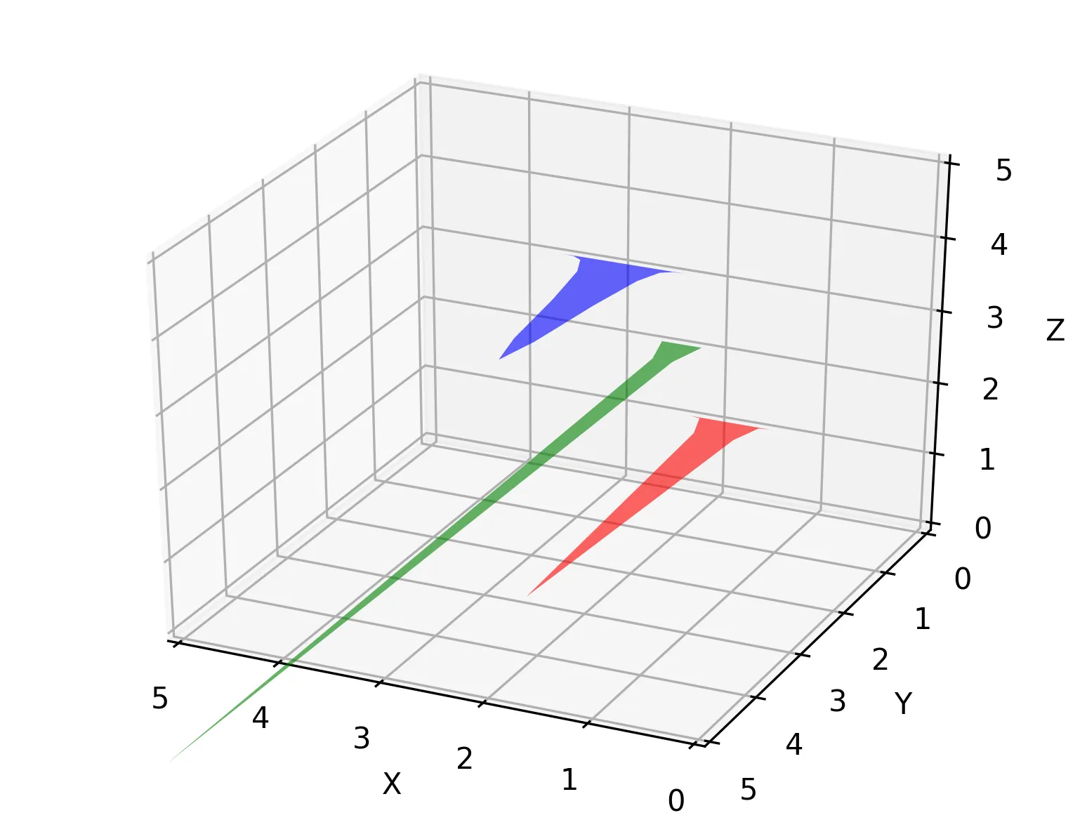
现在，我想用正态分布替换这四个图表（理想情况下形成连续线条）。

我已在此处创建了分布：

def get_xs(lwr_bound = -4, upr_bound = 4, n = 80):
    """ generates the x space betwee lwr_bound and upr_bound so that it has n intermediary steps """
    xs = np.arange(lwr_bound, upr_bound, (upr_bound - lwr_bound) / n) # x space -- number of points on l/r dimension
    return(xs)

xs = get_xs()

dists = [1, 2, 3, 4]

def get_distribution_params(list_):
    """ generates the distribution parameters (mu and sigma) for len(list_) distributions"""
    mus = []
    sigmas = []
    for i in range(len(dists)):
        mus.append(round((i + 1) + 0.1 * np.random.randint(0,10), 3))
        sigmas.append(round((i + 1) * .01 * np.random.randint(0,10), 3))
    return mus, sigmas

mus, sigmas = get_distribution_params(dists)

def get_distributions(list_, xs, mus, sigmas):
    """ generates len(list_) normal distributions, with different mu and sigma values """
    distributions = [] # distributions

    for i in range(len(list_)):
        x_ = xs
        z_ = norm.pdf(xs, loc = mus[i], scale = sigmas[0])
        distributions.append(list(zip(x_, z_)))
        #print(x_[60], z_[60])

    return distributions

distributions = get_distributions(list_ = dists, xs = xs, mus = mus, sigmas = sigmas)

但是将它们添加到代码中（使用poly = PolyCollection(distributions, ...)和ax.add_collection3d(poly，zs=distributions，zdir='z')）会抛出一个ValueError (ValueError：输入操作数的维度超出了轴重映射的允许范围)，我无法解决。

- Ivo

---

请添加完整的非工作示例，包括导入，规范缺失和主题=分布？ - Joe

Answer 1

这个错误是由于将 distributions 传递给了 zs，而 zs 期望在 PolyCollection 中的 verts 形状为 MxNx2 时，传递给 zs 的对象形状为 M。因此当它到达这个检查点时会出现错误。

cpdef ndarray broadcast_to(ndarray array, shape):
    # ...
    if array.ndim < len(shape):
        raise ValueError(
            'input operand has more dimensions than allowed by the axis '
            'remapping')
    # ...

在底层的numpy代码中，出现了错误。我认为这是因为期望的维度数（array.ndim）小于zs的维度数（len(shape)）。它期望一个形状为(4,)的数组，但接收到一个形状为(4, 80, 2)的数组。

可以通过使用正确形状的数组来解决此错误 - 例如原始示例中的zs或您代码中的dists。使用zs=dists并调整x、y和z的轴限制为[0,5]，得到：

这看起来有点奇怪，有两个原因：

1. z_ = norm.pdf(xs, loc = mus[i], scale = sigmas[0]) 中有一个拼写错误，导致所有分布的标准差都相同，应该是 z_ = norm.pdf(xs, loc = mus[i], scale = sigmas[i])
2. 视角问题：分布以正 xz 平面为基础，这也是我们观察的平面。

通过 ax.view_init 更改视角会得到更清晰的图像：

---

编辑

这里是生成所示图形的完整代码，

from mpl_toolkits.mplot3d import Axes3D
from matplotlib.collections import PolyCollection
import matplotlib.pyplot as plt
import matplotlib.colors as mcolors
import numpy as np
from scipy.stats import norm

np.random.seed(8)
def get_xs(lwr_bound = -4, upr_bound = 4, n = 80):
    return np.arange(lwr_bound, upr_bound, (upr_bound - lwr_bound) / n)

def get_distribution_params(list_):
    mus = [round((i+1) + 0.1 * np.random.randint(0,10), 3) for i in range(len(dists))]
    sigmas = [round((i+1) * .01 * np.random.randint(0,10), 3) for i in range(len(dists))]
    return mus, sigmas

def get_distributions(list_, xs, mus, sigmas):
    return [list(zip(xs, norm.pdf(xs, loc=mus[i], scale=sigmas[i] if sigmas[i] != 0.0 
            else 0.1))) for i in range(len(list_))]

dists = [1, 2, 3, 4]
xs = get_xs()
mus, sigmas = get_distribution_params(dists)
distributions = get_distributions(dists, xs, mus, sigmas)

fc = [mcolors.to_rgba('r', alpha=0.6), mcolors.to_rgba('g', alpha=0.6), 
      mcolors.to_rgba('b', alpha=0.6), mcolors.to_rgba('y', alpha=0.6)]

poly = PolyCollection(distributions, fc=fc)
fig = plt.figure()
ax = fig.gca(projection='3d')
ax.add_collection3d(poly, zs=np.array(dists).astype(float), zdir='z')
ax.view_init(azim=115)
ax.set_zlim([0, 5])
ax.set_ylim([0, 5])
ax.set_xlim([0, 5])

我根据您在问题中提供的代码进行了修改，以便更简洁并与通常的样式更一致。

---

注意 - 您提供的示例代码将根据 np.random.seed() 失败，为确保其正常工作，我在调用 norm.pdf 时添加了一个检查，以确保比例尺是非零的: scale = sigma[i] if sigma[i] != 0.0 else 0.1。

- William Miller

---

嗨，William，非常感谢您的回复！我无法完全重现您的代码（即不理解应在何处包含哪些片段），因为进一步的错误让我认为我做错了。您能澄清一下您建议的代码是什么样子吗？:) 非常感谢！ - Ivo

@Ivo 我很乐意帮忙，但可能需要几天时间才能处理好... 如果我几天内没有更新答案，请随时提醒我。 - William Miller

你有时间看这个了吗？ :) - Ivo

@Ivo 我还没有完成 - 我有点忙，但我计划很快完成。谢谢你提醒我。 - William Miller

@Ivo 我已添加了我用来生成所示图形的完整代码 - 希望这将有助于澄清问题。 - William Miller

Answer 2

使用 ax.add_collection3d(poly, zs=dists, zdir='z') 替代 ax.add_collection3d(poly, zs=distributions, zdir='z') 应该能解决这个问题。

---

此外，您可能想要替换：

。

def get_xs(lwr_bound = -4, upr_bound = 4, n = 80):
    """ generates the x space betwee lwr_bound and upr_bound so that it has n intermediary steps """
    xs = np.arange(lwr_bound, upr_bound, (upr_bound - lwr_bound) / n) # x space -- number of points on l/r dimension
    return(xs)

xs = get_xs()

由

xs = np.linspace(-4, 4, 80)

---

此外，我认为在该行中scale = sigmas[0]实际上应该是scale = sigmas[i]。

z_ = norm.pdf(xs, loc = mus[i], scale = sigmas[0])

---

最后，我认为您应该适当调整xlim、ylim和zlim，因为您在与参考代码进行比较时交换了绘图的y和z维度，并改变了其比例。

- Maxpxt