在 ggplot 的 geom_curve 线中添加标签

Question

在 ggplot 的 geom_curve 线中添加标签

9

有没有办法在geom_curve线的中心或附近添加标签？目前，我只能通过对曲线的起点或终点进行标记来实现。

library(tidyverse)
library(ggrepel)

df <- data.frame(x1 = 1, y1 = 1, x2 = 2, y2 = 3, details = "Object Name")

ggplot(df, aes(x = x1, y = y1, label = details)) +
  geom_point(size = 4) +
  geom_point(aes(x = x2, y = y2),
             pch = 17, size = 4) +
  geom_curve(aes(x = x1, y = y1, xend = x2, yend = y2)) +
  geom_label(nudge_y = 0.05) +
  geom_label_repel(box.padding = 2)

我希望能找到一种自动标记曲线的方法，标记在x=1.75，y=1.5附近的坐标。是否有我尚未发现的解决方案？我的图表比较繁忙，标记原点会使其更难以观察，而标记弧线则会产生更清晰的输出。

- Watanake

2个回答

1

也许注释会有所帮助（参见：http://ggplot2.tidyverse.org/reference/annotate.html）。

library(tidyverse)
library(ggrepel)

df <- data.frame(x1 = 1, y1 = 1, x2 = 2, y2 = 3, details = "Object Name")

ggplot(df, aes(x = x1, y = y1, label = details)) +
  geom_point(size = 4) +
  geom_point(aes(x = x2, y = y2),
             pch = 17, size = 4) +
  geom_curve(aes(x = x1, y = y1, xend = x2, yend = y2)) +
  geom_label(nudge_y = 0.05) +
  geom_label_repel(box.padding = 2) +
  annotate("label", x=1.75, y=1.5, label=df$details)

- Wolfgang Arnold

是的，我认为annotate可能是要使用的函数，但为了可扩展性，我需要一种计算每个感兴趣的弧线中点位置的方法。手动筛选不适合这个项目。但也许关键在于一个几何问题，如何找到每个geom_curve弧线的中点。 - Watanake

网页内容由stack overflow 提供, 点击上面的

可以查看英文原文，
原文链接

- Watanake · Accepted Answer

我已经找到了解决这个问题的方法。它很大而笨重，但是有效。

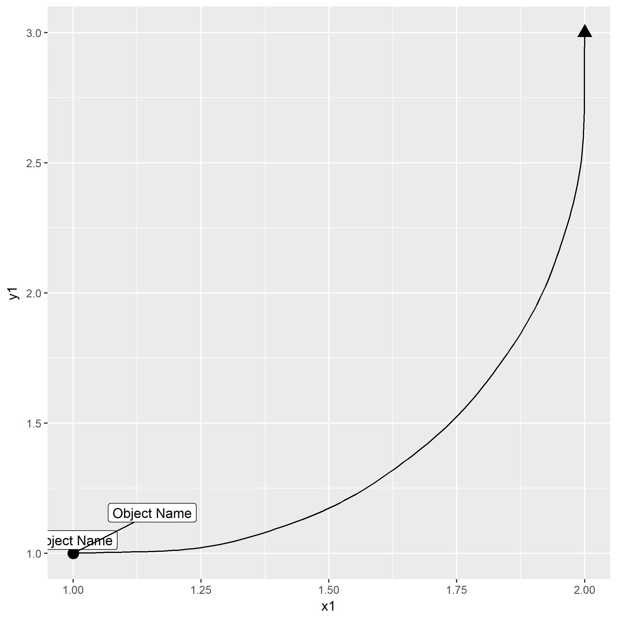
核心问题是geom_curve()不会绘制一个固定的路径，而是随着绘图窗口的纵横比例进行移动和缩放。因此，除了使用coord_fixed(ratio=1)锁定纵横比例之外，我很难预测geom_curve()段的中点位置。

因此，我开始寻找曲线的中点，然后强制曲线通过这个点，之后我会给它贴标签。为了找到中点，我不得不从grid package中复制两个函数。

library(grid)
library(tidyverse)
library(ggrepel)

# Find origin of rotation
# Rotate around that origin
calcControlPoints <- function(x1, y1, x2, y2, curvature, angle, ncp,
                              debug=FALSE) {
  # Negative curvature means curve to the left
  # Positive curvature means curve to the right
  # Special case curvature = 0 (straight line) has been handled
  xm <- (x1 + x2)/2
  ym <- (y1 + y2)/2
  dx <- x2 - x1
  dy <- y2 - y1
  slope <- dy/dx

  # Calculate "corner" of region to produce control points in
  # (depends on 'angle', which MUST lie between 0 and 180)
  # Find by rotating start point by angle around mid point
  if (is.null(angle)) {
    # Calculate angle automatically
    angle <- ifelse(slope < 0,
                    2*atan(abs(slope)),
                    2*atan(1/slope))
  } else {
    angle <- angle/180*pi
  }
  sina <- sin(angle)
  cosa <- cos(angle)
  # FIXME:  special case of vertical or horizontal line ?
  cornerx <- xm + (x1 - xm)*cosa - (y1 - ym)*sina
  cornery <- ym + (y1 - ym)*cosa + (x1 - xm)*sina

  # Debugging
  if (debug) {
    grid.points(cornerx, cornery, default.units="inches",
                pch=16, size=unit(3, "mm"),
                gp=gpar(col="grey"))
  }

  # Calculate angle to rotate region by to align it with x/y axes
  beta <- -atan((cornery - y1)/(cornerx - x1))
  sinb <- sin(beta)
  cosb <- cos(beta)
  # Rotate end point about start point to align region with x/y axes
  newx2 <- x1 + dx*cosb - dy*sinb
  newy2 <- y1 + dy*cosb + dx*sinb

  # Calculate x-scale factor to make region "square"
  # FIXME:  special case of vertical or horizontal line ?
  scalex <- (newy2 - y1)/(newx2 - x1)
  # Scale end points to make region "square"
  newx1 <- x1*scalex
  newx2 <- newx2*scalex

  # Calculate the origin in the "square" region
  # (for rotating start point to produce control points)
  # (depends on 'curvature')
  # 'origin' calculated from 'curvature'
  ratio <- 2*(sin(atan(curvature))^2)
  origin <- curvature - curvature/ratio
  # 'hand' also calculated from 'curvature'
  if (curvature > 0)
    hand <- "right"
  else
    hand <- "left"
  oxy <- calcOrigin(newx1, y1, newx2, newy2, origin, hand)
  ox <- oxy$x
  oy <- oxy$y

  # Calculate control points
  # Direction of rotation depends on 'hand'
  dir <- switch(hand,
                left=-1,
                right=1)
  # Angle of rotation depends on location of origin
  maxtheta <- pi + sign(origin*dir)*2*atan(abs(origin))
  theta <- seq(0, dir*maxtheta,
               dir*maxtheta/(ncp + 1))[c(-1, -(ncp + 2))]
  costheta <- cos(theta)
  sintheta <- sin(theta)
  # May have BOTH multiple end points AND multiple
  # control points to generate (per set of end points)
  # Generate consecutive sets of control points by performing
  # matrix multiplication
  cpx <- ox + ((newx1 - ox) %*% t(costheta)) -
    ((y1 - oy) %*% t(sintheta))
  cpy <- oy + ((y1 - oy) %*% t(costheta)) +
    ((newx1 - ox) %*% t(sintheta))

  # Reverse transformations (scaling and rotation) to
  # produce control points in the original space
  cpx <- cpx/scalex
  sinnb <- sin(-beta)
  cosnb <- cos(-beta)
  finalcpx <- x1 + (cpx - x1)*cosnb - (cpy - y1)*sinnb
  finalcpy <- y1 + (cpy - y1)*cosnb + (cpx - x1)*sinnb

  # Debugging
  if (debug) {
    ox <- ox/scalex
    fox <- x1 + (ox - x1)*cosnb - (oy - y1)*sinnb
    foy <- y1 + (oy - y1)*cosnb + (ox - x1)*sinnb
    grid.points(fox, foy, default.units="inches",
                pch=16, size=unit(1, "mm"),
                gp=gpar(col="grey"))
    grid.circle(fox, foy, sqrt((ox - x1)^2 + (oy - y1)^2),
                default.units="inches",
                gp=gpar(col="grey"))
  }

  list(x=as.numeric(t(finalcpx)), y=as.numeric(t(finalcpy)))
}

calcOrigin <- function(x1, y1, x2, y2, origin, hand) {
  # Positive origin means origin to the "right"
  # Negative origin means origin to the "left"
  xm <- (x1 + x2)/2
  ym <- (y1 + y2)/2
  dx <- x2 - x1
  dy <- y2 - y1
  slope <- dy/dx
  oslope <- -1/slope
  # The origin is a point somewhere along the line between
  # the end points, rotated by 90 (or -90) degrees
  # Two special cases:
  # If slope is non-finite then the end points lie on a vertical line, so
  # the origin lies along a horizontal line (oslope = 0)
  # If oslope is non-finite then the end points lie on a horizontal line,
  # so the origin lies along a vertical line (oslope = Inf)
  tmpox <- ifelse(!is.finite(slope),
                  xm,
                  ifelse(!is.finite(oslope),
                         xm + origin*(x2 - x1)/2,
                         xm + origin*(x2 - x1)/2))
  tmpoy <- ifelse(!is.finite(slope),
                  ym + origin*(y2 - y1)/2,
                  ifelse(!is.finite(oslope),
                         ym,
                         ym + origin*(y2 - y1)/2))
  # ALWAYS rotate by -90 about midpoint between end points
  # Actually no need for "hand" because "origin" also
  # encodes direction
  # sintheta <- switch(hand, left=-1, right=1)
  sintheta <- -1
  ox <- xm - (tmpoy - ym)*sintheta
  oy <- ym + (tmpox - xm)*sintheta

  list(x=ox, y=oy)
}

有了那个条件，我计算了每个记录的中点。

df <- data.frame(x1 = 1, y1 = 1, x2 = 10, y2 = 10, details = "Object Name")

df_mid <- df %>% 
  mutate(midx = calcControlPoints(x1, y1, x2, y2, 
                                  angle = 130, 
                                  curvature = 0.5, 
                                  ncp = 1)$x) %>% 
  mutate(midy = calcControlPoints(x1, y1, x2, y2, 
                                  angle = 130, 
                                  curvature = 0.5, 
                                  ncp = 1)$y)

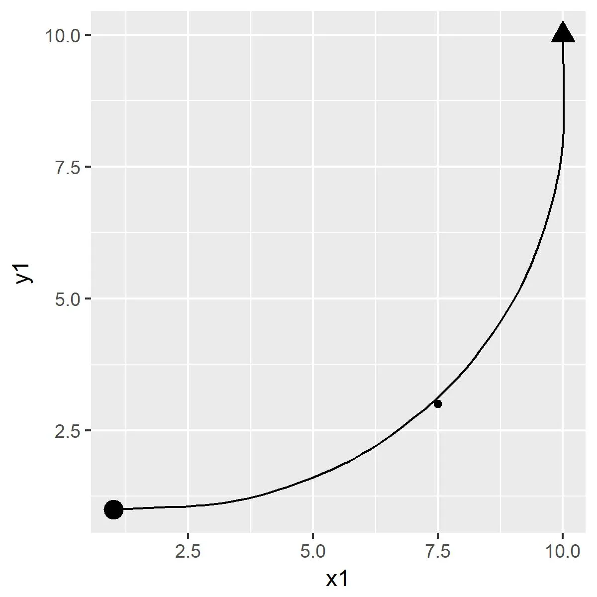
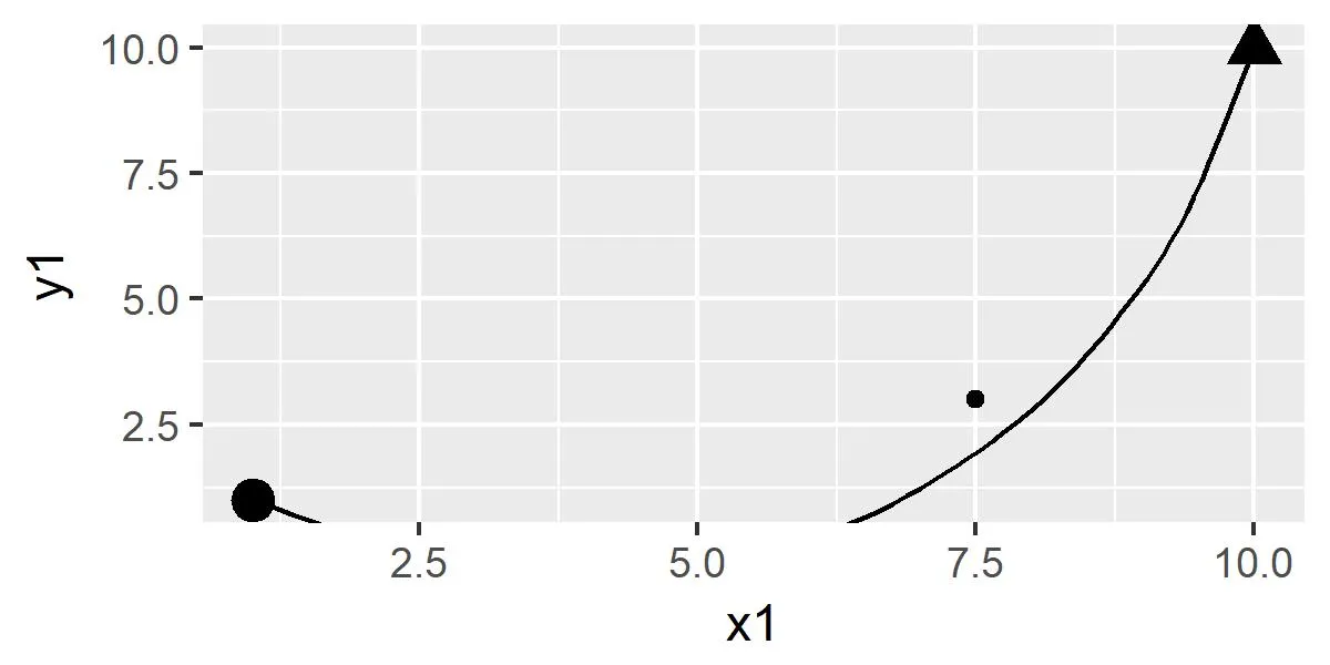
我接着画出这张图，但是绘制了两条分开的曲线。一条从原点到计算出的中点，另一条从中点到目的地。找到中点和绘制这些曲线的角度和曲率设置很棘手，以确保结果不明显看起来像两个不同的曲线。

ggplot(df_mid, aes(x = x1, y = y1)) +
  geom_point(size = 4) +
  geom_point(aes(x = x2, y = y2),
             pch = 17, size = 4) +
  geom_curve(aes(x = x1, y = y1, xend = midx, yend = midy),
             curvature = 0.25, angle = 135) +
  geom_curve(aes(x = midx, y = midy, xend = x2, yend = y2),
             curvature = 0.25, angle = 45) +
  geom_label_repel(aes(x = midx, y = midy, label = details),
                   box.padding = 4,
                   nudge_x = 0.5,
                   nudge_y = -2)

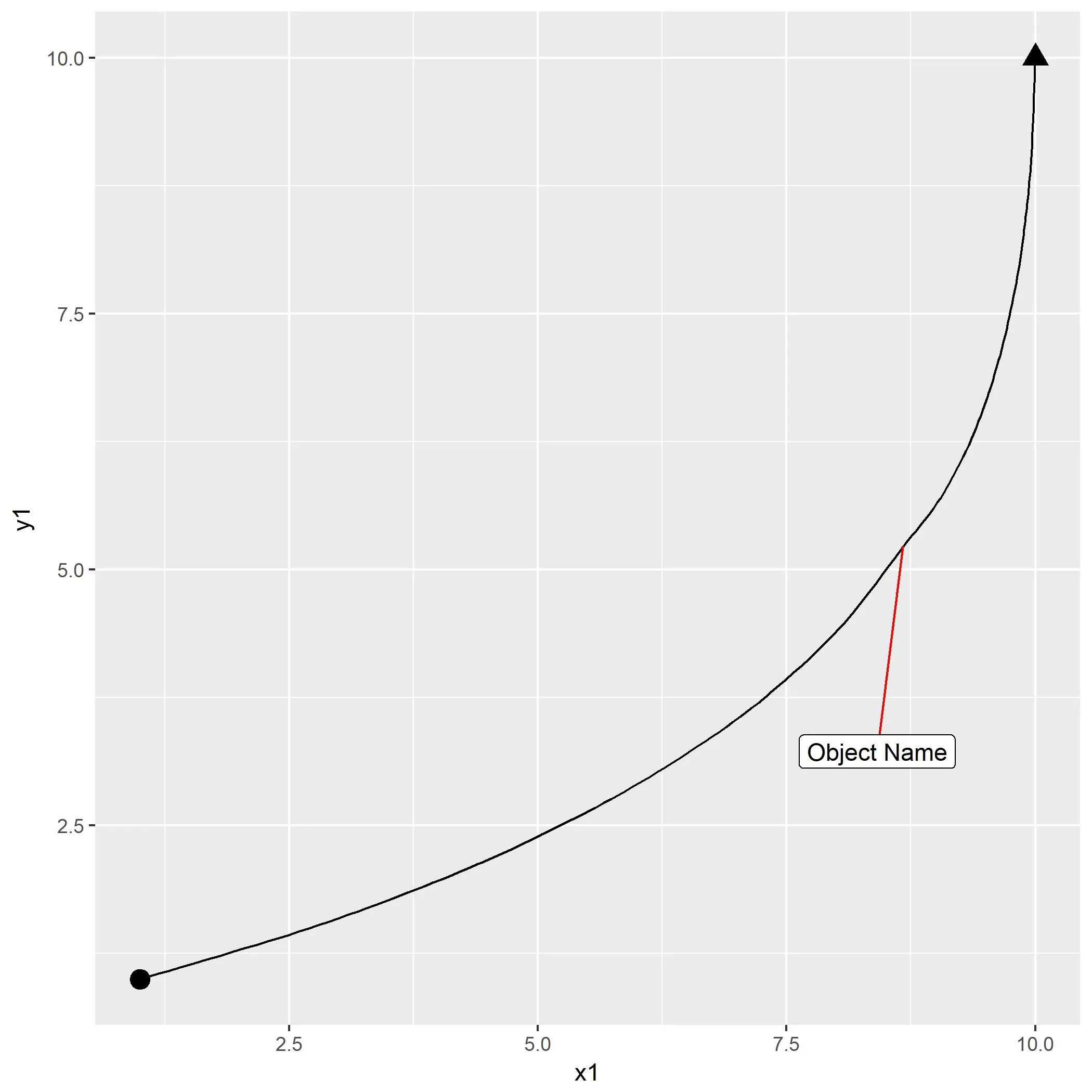
尽管答案并不理想或优雅，但它可以适用于大量记录。