在三维空间中，一条线曲线的样条插值系数

Question

我是Python新手。在由一组给定点定义的三维空间中，我有一条曲线。有人能够建议我如何使用scipy包中的样条(spline)函数进行插值(interpolate)，从而像MATLAB中的spline.coeff函数一样获取曲线的样条系数吗？谢谢!

编辑：

我已经使用了

tck = interpolate.SmoothBivariateSpline(pts2[:,0], pts2[:,1], pts2[:,2])
test_pts = pts2[:,2]-tck.ev(pts2[:,0], pts2[:,1])
print test_pts

但这似乎只适用于曲面，而不适用于线曲线。pts2是一个包含点坐标的Nx3 numpy array。

好的，我弄清楚了我做错了什么。我的输入点太少了。现在我有另一个问题。函数get_coeffs应该返回每个节点处的样条系数。这些系数以何种顺序返回？我有一个79个tx和79个ty的数组，表示节点，当我调用函数来调用这些节点时，我得到一个1x5625的数组。

- Yannis

---

我使用了tck = interpolate.SmoothBivariateSpline(pts2[:,0],pts2[:,1],pts2[:,2])，但这似乎是用于曲面而不是线曲线的。 pts2是一个包含点坐标的Nx3 numpy数组。 - Yannis

你能否编辑你的帖子并添加这些信息呢？这将有助于其他读者。 - Paco

代码： tck = interpolate.SmoothBivariateSpline(pts2[:,0],pts2[:,1],pts2[:,2])test_pts = pts2[:,2]-tck.ev(pts2[:,0],pts2[:,1]) print test_pts - Yannis

好的，我弄清楚了我的错误。我的输入点太少了。 现在我有另一个问题。 函数get_coeffs应该在每个节点返回样条系数。 这些系数以什么顺序返回？ 我有一个由79个tx和79个ty组成的数组，表示节点，当我调用函数来调用节点时，我得到一个1x5625的数组。 - Yannis

如果您找到了解决问题的答案，请将其发布为答案。对于新问题，请开启另一个提问。 - Paco

Answer 1

我也是Python的新手，但最近我的搜索让我找到了一个非常有用的scipy插值教程。从我对此的阅读中，我认为BivariateSpline类/函数族旨在插值3D表面而不是3D曲线。

对于我的3D曲线拟合问题（我认为与您的非常相似，但还想平滑噪声），我最终使用了scipy.interpolate.splprep（不要与scipy.interpolate.splrep混淆）。从上面链接的教程中，您正在寻找的样条系数由splprep返回。

正常输出是一个3元组（t，c，k），其中包含结点t，系数c和样条的阶数k。

文档将这些过程函数称为“较旧的、非面向对象的FITPACK包装”，与“较新的、面向对象的”UnivariateSpline和BivariateSpline类形成对比。我本人更喜欢“较新的、面向对象的”方式，但据我所知，UnivariateSpline只处理1-D情况，而splprep直接处理N-D数据。以下是我用来测试这些函数的简单测试案例：

import numpy as np
import matplotlib.pyplot as plt
from scipy import interpolate
from mpl_toolkits.mplot3d import Axes3D


# 3D example
total_rad = 10
z_factor = 3
noise = 0.1

num_true_pts = 200
s_true = np.linspace(0, total_rad, num_true_pts)
x_true = np.cos(s_true)
y_true = np.sin(s_true)
z_true = s_true/z_factor

num_sample_pts = 80
s_sample = np.linspace(0, total_rad, num_sample_pts)
x_sample = np.cos(s_sample) + noise * np.random.randn(num_sample_pts)
y_sample = np.sin(s_sample) + noise * np.random.randn(num_sample_pts)
z_sample = s_sample/z_factor + noise * np.random.randn(num_sample_pts)

tck, u = interpolate.splprep([x_sample,y_sample,z_sample], s=2)
x_knots, y_knots, z_knots = interpolate.splev(tck[0], tck)
u_fine = np.linspace(0,1,num_true_pts)
x_fine, y_fine, z_fine = interpolate.splev(u_fine, tck)

fig2 = plt.figure(2)
ax3d = fig2.add_subplot(111, projection='3d')
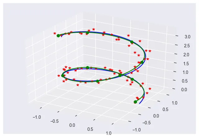
ax3d.plot(x_true, y_true, z_true, 'b')
ax3d.plot(x_sample, y_sample, z_sample, 'r*')
ax3d.plot(x_knots, y_knots, z_knots, 'go')
ax3d.plot(x_fine, y_fine, z_fine, 'g')
fig2.show()
plt.show()

- neal