卡尔曼滤波器与不同时间步长的应用

Question

我有一些数据，表示从两个不同的传感器测量得到的物体位置。因此，我需要进行传感器融合。更困难的问题是，每个传感器的数据基本上以随机时间到达。我想使用pykalman来融合和平滑数据。pykalman如何处理变量时间戳数据？

简化的样本数据如下：

import pandas as pd
data={'time':\
['10:00:00.0','10:00:01.0','10:00:05.2','10:00:07.5','10:00:07.5','10:00:12.0','10:00:12.5']\
,'X':[10,10.1,20.2,25.0,25.1,35.1,35.0],'Y':[20,20.2,41,45,47,75.0,77.2],\
'Sensor':[1,2,1,1,2,1,2]}

df=pd.DataFrame(data,columns=['time','X','Y','Sensor'])
df.time=pd.to_datetime(df.time)
df=df.set_index('time')

并且这个：

df
Out[130]: 
                            X     Y  Sensor
time                                       
2017-12-01 10:00:00.000  10.0  20.0       1
2017-12-01 10:00:01.000  10.1  20.2       2
2017-12-01 10:00:05.200  20.2  41.0       1
2017-12-01 10:00:07.500  25.0  45.0       1
2017-12-01 10:00:07.500  25.1  47.0       2
2017-12-01 10:00:12.000  35.1  75.0       1
2017-12-01 10:00:12.500  35.0  77.2       2

对于传感器融合问题，我认为可以重塑数据，使得它包含位置X1、Y1、X2和Y2以及一些缺失值，而不仅是X和Y坐标。（这个问题相关： https://stackoverflow.com/questions/47386426/2-sensor-readings-fusion-yaw-pitch）

那么我的数据看起来就像这样：

df['X1']=df.X[df.Sensor==1]
df['Y1']=df.Y[df.Sensor==1]
df['X2']=df.X[df.Sensor==2]
df['Y2']=df.Y[df.Sensor==2]
df
Out[132]: 
                            X     Y  Sensor    X1    Y1    X2    Y2
time                                                               
2017-12-01 10:00:00.000  10.0  20.0       1  10.0  20.0   NaN   NaN
2017-12-01 10:00:01.000  10.1  20.2       2   NaN   NaN  10.1  20.2
2017-12-01 10:00:05.200  20.2  41.0       1  20.2  41.0   NaN   NaN
2017-12-01 10:00:07.500  25.0  45.0       1  25.0  45.0  25.1  47.0
2017-12-01 10:00:07.500  25.1  47.0       2  25.0  45.0  25.1  47.0
2017-12-01 10:00:12.000  35.1  75.0       1  35.1  75.0   NaN   NaN
2017-12-01 10:00:12.500  35.0  77.2       2   NaN   NaN  35.0  77.2

pykalman的文档表明它可以处理缺失数据，但这是正确的吗？

但是，pykalman的文档并没有很清楚地说明变量时间问题。文档只是说：

“卡尔曼滤波器和卡尔曼平滑器都能够使用随时间变化的参数。为了使用此功能，只需沿着其第一个轴传入长度为n_timesteps的数组：”

>>> transition_offsets = [[-1], [0], [1], [2]]
>>> kf = KalmanFilter(transition_offsets=transition_offsets, n_dim_obs=1)

我没有找到使用pykalman Smoother处理变时间步的示例。因此，任何指导、示例，甚至是使用上述数据的示例都将非常有帮助。

不一定要使用pykalman，但似乎这是一个很有用的工具来平滑这些数据。

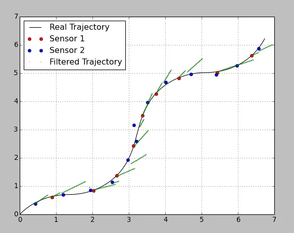
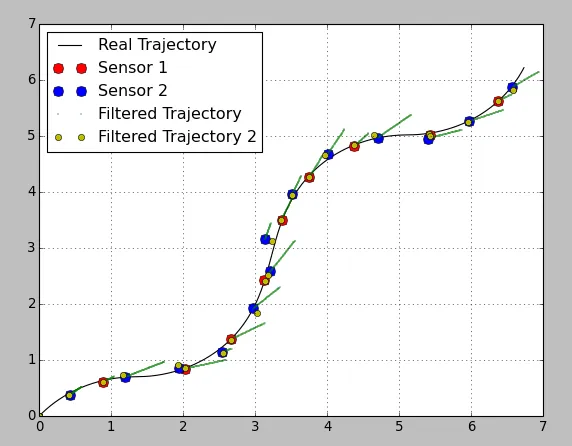
***** 下面添加了额外的代码 @Anton 我制作了一个使用smooth函数的有用代码版本。奇怪的是它似乎将每个观测值视为同等重要，并使轨迹通过每个观测点。即使传感器方差值之间有很大的差异。我期望在5.4,5.0点附近，过滤后的轨迹会更靠近传感器1的点，因为传感器1的方差较低。然而轨迹确切地经过每个点，并进行大幅度转向以抵达那里。

from pykalman import KalmanFilter
import numpy as np
import matplotlib.pyplot as plt

# reading data (quick and dirty)
Time=[]
RefX=[]
RefY=[]
Sensor=[]
X=[]
Y=[]

for line in open('data/dataset_01.csv'):
    f1, f2, f3, f4, f5, f6 = line.split(';')
    Time.append(float(f1))
    RefX.append(float(f2))
    RefY.append(float(f3))
    Sensor.append(float(f4))
    X.append(float(f5))
    Y.append(float(f6))

# Sensor 1 has a higher precision (max error = 0.1 m)
# Sensor 2 has a lower precision (max error = 0.3 m)

# Variance definition through 3-Sigma rule
Sensor_1_Variance = (0.1/3)**2;
Sensor_2_Variance = (0.3/3)**2;

# Filter Configuration

# time step
dt = Time[2] - Time[1]

# transition_matrix  
F = [[1,  0,  dt,   0], 
     [0,  1,   0,  dt],
     [0,  0,   1,   0],
     [0,  0,   0,   1]]   

# observation_matrix   
H = [[1, 0, 0, 0],
     [0, 1, 0, 0]]

# transition_covariance 
Q = [[1e-4,     0,     0,     0], 
     [   0,  1e-4,     0,     0],
     [   0,     0,  1e-4,     0],
     [   0,     0,     0,  1e-4]] 

# observation_covariance 
R_1 = [[Sensor_1_Variance, 0],
       [0, Sensor_1_Variance]]

R_2 = [[Sensor_2_Variance, 0],
       [0, Sensor_2_Variance]]

# initial_state_mean
X0 = [0,
      0,
      0,
      0]

# initial_state_covariance - assumed a bigger uncertainty in initial velocity
P0 = [[  0,    0,   0,   0], 
      [  0,    0,   0,   0],
      [  0,    0,   1,   0],
      [  0,    0,   0,   1]]

n_timesteps = len(Time)
n_dim_state = 4
filtered_state_means = np.zeros((n_timesteps, n_dim_state))
filtered_state_covariances = np.zeros((n_timesteps, n_dim_state, n_dim_state))

import numpy.ma as ma

obs_cov=np.zeros([n_timesteps,2,2])
obs=np.zeros([n_timesteps,2])

for t in range(n_timesteps):
    if Sensor[t] == 0:
        obs[t]=None
    else:
        obs[t] = [X[t], Y[t]]
        if Sensor[t] == 1:
            obs_cov[t] = np.asarray(R_1)
        else:
            obs_cov[t] = np.asarray(R_2)

ma_obs=ma.masked_invalid(obs)

ma_obs_cov=ma.masked_invalid(obs_cov)

# Kalman-Filter initialization
kf = KalmanFilter(transition_matrices = F, 
                  observation_matrices = H, 
                  transition_covariance = Q, 
                  observation_covariance = ma_obs_cov, # the covariance will be adapted depending on Sensor_ID
                  initial_state_mean = X0, 
                  initial_state_covariance = P0)

filtered_state_means, filtered_state_covariances=kf.smooth(ma_obs)


# extracting the Sensor update points for the plot        
Sensor_1_update_index = [i for i, x in enumerate(Sensor) if x == 1]    
Sensor_2_update_index = [i for i, x in enumerate(Sensor) if x == 2]     

Sensor_1_update_X = [ X[i] for i in Sensor_1_update_index ]        
Sensor_1_update_Y = [ Y[i] for i in Sensor_1_update_index ]   

Sensor_2_update_X = [ X[i] for i in Sensor_2_update_index ]        
Sensor_2_update_Y = [ Y[i] for i in Sensor_2_update_index ] 

# plot of the resulted trajectory
plt.plot(RefX, RefY, "k-", label="Real Trajectory")
plt.plot(Sensor_1_update_X, Sensor_1_update_Y, "ro", label="Sensor 1")
plt.plot(Sensor_2_update_X, Sensor_2_update_Y, "bo", label="Sensor 2")
plt.plot(filtered_state_means[:, 0], filtered_state_means[:, 1], "g.", label="Filtered Trajectory", markersize=1)
plt.grid()
plt.legend(loc="upper left")
plt.show()    

- Adam

---

我认为随机时间问题没有任何问题。您有模型来预测状态和测量值来纠正预测的状态。如果有时候测量值丢失，您仍然可以进行预测。您能否提供更多关于您的模型的数据，这样我就可以尝试解决这个问题？ - Anton

使用两个未同步的传感器，大多数观测结果将缺失其中一个或另一个测量值。此外，似乎pykalman在任何单个列具有缺失值时都会删除整个观测结果。因此，在上面的示例中，它的行为就像只有一个观测结果。如果需要，我可以添加一些细节。 - Adam

你有关于传感器精度的一些信息吗？你需要定义方差，是吗？而且你必须使用pykalman吗？在Python中设计自己的滤波器并不难。所以如果你提供足够的信息，我可以做到。我喜欢这个话题。 - Anton

上面的最后一行代码，包括transition_offsets，来自于pykalman的手册，而不是我的代码。手册中的示例确实表明它具有默认值。 - Adam

Answer 1

对于卡尔曼滤波器，使用恒定时间步长来表示输入数据是有用的。由于传感器发送数据是随机的，因此您可以定义系统中最小的有效时间步长，并使用此步长离散化时间轴。

例如，您的一个传感器大约每0.2秒发送一次数据，第二个传感器每0.5秒发送一次数据。因此，最小时间步长可以是0.01秒（在这里，您需要在计算时间和所需精度之间找到平衡）。

您的数据将如下所示：

Time    Sensor  X       Y
0,52        0   0       0
0,53        1   0,3417  0,2988
0,54        0   0       0
0,56        0   0       0
0,57        0   0       0
0,55        0   0       0
0,58        0   0       0
0,59        2   0,4247  0,3779
0,60        0   0       0
0,61        0   0       0
0,62        0   0       0

现在，根据您的观测结果，您需要调用Pykalman函数filter_update。如果没有观测结果，滤波器将基于上一个状态预测下一个状态。如果有观测结果，则会纠正系统状态。

可能您的传感器精度不同。因此，您可以根据传感器方差指定观测协方差。

为了演示这个想法，我生成了一个2D轨迹，并随机放置了两个具有不同准确度的传感器的测量值。

Sensor1: mean update time = 1.0s; max error = 0.1m;
Sensor2: mean update time = 0.7s; max error = 0.3m;

以下是结果：

我特意选择了非常糟糕的参数，以便可以看到预测和校正步骤。在传感器更新之间，滤波器基于上一步的恒定速度预测轨迹。一旦有更新，滤波器根据传感器方差校正位置。第二个传感器的精度非常低，因此它以较低的权重影响系统。

这是我的Python代码：

from pykalman import KalmanFilter
import numpy as np
import matplotlib.pyplot as plt

# reading data (quick and dirty)
Time=[]
RefX=[]
RefY=[]
Sensor=[]
X=[]
Y=[]

for line in open('data/dataset_01.csv'):
    f1, f2, f3, f4, f5, f6 = line.split(';')
    Time.append(float(f1))
    RefX.append(float(f2))
    RefY.append(float(f3))
    Sensor.append(float(f4))
    X.append(float(f5))
    Y.append(float(f6))

# Sensor 1 has a higher precision (max error = 0.1 m)
# Sensor 2 has a lower precision (max error = 0.3 m)

# Variance definition through 3-Sigma rule
Sensor_1_Variance = (0.1/3)**2;
Sensor_2_Variance = (0.3/3)**2;

# Filter Configuration

# time step
dt = Time[2] - Time[1]

# transition_matrix  
F = [[1,  0,  dt,   0], 
     [0,  1,   0,  dt],
     [0,  0,   1,   0],
     [0,  0,   0,   1]]   

# observation_matrix   
H = [[1, 0, 0, 0],
     [0, 1, 0, 0]]

# transition_covariance 
Q = [[1e-4,     0,     0,     0], 
     [   0,  1e-4,     0,     0],
     [   0,     0,  1e-4,     0],
     [   0,     0,     0,  1e-4]] 

# observation_covariance 
R_1 = [[Sensor_1_Variance, 0],
       [0, Sensor_1_Variance]]

R_2 = [[Sensor_2_Variance, 0],
       [0, Sensor_2_Variance]]

# initial_state_mean
X0 = [0,
      0,
      0,
      0]

# initial_state_covariance - assumed a bigger uncertainty in initial velocity
P0 = [[  0,    0,   0,   0], 
      [  0,    0,   0,   0],
      [  0,    0,   1,   0],
      [  0,    0,   0,   1]]

n_timesteps = len(Time)
n_dim_state = 4
filtered_state_means = np.zeros((n_timesteps, n_dim_state))
filtered_state_covariances = np.zeros((n_timesteps, n_dim_state, n_dim_state))

# Kalman-Filter initialization
kf = KalmanFilter(transition_matrices = F, 
                  observation_matrices = H, 
                  transition_covariance = Q, 
                  observation_covariance = R_1, # the covariance will be adapted depending on Sensor_ID
                  initial_state_mean = X0, 
                  initial_state_covariance = P0)


# iterative estimation for each new measurement
for t in range(n_timesteps):
    if t == 0:
        filtered_state_means[t] = X0
        filtered_state_covariances[t] = P0
    else:

        # the observation and its covariance have to be switched depending on Sensor_Id 
        #     Sensor_ID == 0: no observation
        #     Sensor_ID == 1: Sensor 1
        #     Sensor_ID == 2: Sensor 2

        if Sensor[t] == 0:
            obs = None
            obs_cov = None
        else:
            obs = [X[t], Y[t]]

            if Sensor[t] == 1:
                obs_cov = np.asarray(R_1)
            else:
                obs_cov = np.asarray(R_2)

        filtered_state_means[t], filtered_state_covariances[t] = (
        kf.filter_update(
            filtered_state_means[t-1],
            filtered_state_covariances[t-1],
            observation = obs,
            observation_covariance = obs_cov)
        )

# extracting the Sensor update points for the plot        
Sensor_1_update_index = [i for i, x in enumerate(Sensor) if x == 1]    
Sensor_2_update_index = [i for i, x in enumerate(Sensor) if x == 2]     

Sensor_1_update_X = [ X[i] for i in Sensor_1_update_index ]        
Sensor_1_update_Y = [ Y[i] for i in Sensor_1_update_index ]   

Sensor_2_update_X = [ X[i] for i in Sensor_2_update_index ]        
Sensor_2_update_Y = [ Y[i] for i in Sensor_2_update_index ] 

# plot of the resulted trajectory
plt.plot(RefX, RefY, "k-", label="Real Trajectory")
plt.plot(Sensor_1_update_X, Sensor_1_update_Y, "ro", label="Sensor 1")
plt.plot(Sensor_2_update_X, Sensor_2_update_Y, "bo", label="Sensor 2")
plt.plot(filtered_state_means[:, 0], filtered_state_means[:, 1], "g.", label="Filtered Trajectory", markersize=1)
plt.grid()
plt.legend(loc="upper left")
plt.show()    

我把csv文件放在这里，这样你就可以执行代码了。

希望能对你有所帮助。 更新 关于你提出的变量转移矩阵建议，我认为这取决于传感器的可用性和对估计结果的要求。

下面是使用恒定和可变转移矩阵进行相同估计的图表（我改变了转移协方差矩阵，否则由于高滤波“刚度”，估计结果会很差）： 如您所见，黄色标记的估计位置非常好。但是！在传感器读数之间没有任何信息。使用可变转移矩阵可以避免读数之间的预测步骤，并且不知道系统发生了什么。如果您的读数具有高速率，则可以足够好，但否则可能是一个缺点。

以下是更新后的代码：

from pykalman import KalmanFilter
import numpy as np
import matplotlib.pyplot as plt

# reading data (quick and dirty)
Time=[]
RefX=[]
RefY=[]
Sensor=[]
X=[]
Y=[]

for line in open('data/dataset_01.csv'):
    f1, f2, f3, f4, f5, f6 = line.split(';')
    Time.append(float(f1))
    RefX.append(float(f2))
    RefY.append(float(f3))
    Sensor.append(float(f4))
    X.append(float(f5))
    Y.append(float(f6))

# Sensor 1 has a higher precision (max error = 0.1 m)
# Sensor 2 has a lower precision (max error = 0.3 m)

# Variance definition through 3-Sigma rule
Sensor_1_Variance = (0.1/3)**2;
Sensor_2_Variance = (0.3/3)**2;

# Filter Configuration

# time step
dt = Time[2] - Time[1]

# transition_matrix  
F = [[1,  0,  dt,   0], 
     [0,  1,   0,  dt],
     [0,  0,   1,   0],
     [0,  0,   0,   1]]   

# observation_matrix   
H = [[1, 0, 0, 0],
     [0, 1, 0, 0]]

# transition_covariance 
Q = [[1e-2,     0,     0,     0], 
     [   0,  1e-2,     0,     0],
     [   0,     0,  1e-2,     0],
     [   0,     0,     0,  1e-2]] 

# observation_covariance 
R_1 = [[Sensor_1_Variance, 0],
       [0, Sensor_1_Variance]]

R_2 = [[Sensor_2_Variance, 0],
       [0, Sensor_2_Variance]]

# initial_state_mean
X0 = [0,
      0,
      0,
      0]

# initial_state_covariance - assumed a bigger uncertainty in initial velocity
P0 = [[  0,    0,   0,   0], 
      [  0,    0,   0,   0],
      [  0,    0,   1,   0],
      [  0,    0,   0,   1]]

n_timesteps = len(Time)
n_dim_state = 4

filtered_state_means = np.zeros((n_timesteps, n_dim_state))
filtered_state_covariances = np.zeros((n_timesteps, n_dim_state, n_dim_state))

filtered_state_means2 = np.zeros((n_timesteps, n_dim_state))
filtered_state_covariances2 = np.zeros((n_timesteps, n_dim_state, n_dim_state))

# Kalman-Filter initialization
kf = KalmanFilter(transition_matrices = F, 
                  observation_matrices = H, 
                  transition_covariance = Q, 
                  observation_covariance = R_1, # the covariance will be adapted depending on Sensor_ID
                  initial_state_mean = X0, 
                  initial_state_covariance = P0)

# Kalman-Filter initialization (Different F Matrices depending on DT)
kf2 = KalmanFilter(transition_matrices = F, 
                  observation_matrices = H, 
                  transition_covariance = Q, 
                  observation_covariance = R_1, # the covariance will be adapted depending on Sensor_ID
                  initial_state_mean = X0, 
                  initial_state_covariance = P0)


# iterative estimation for each new measurement
for t in range(n_timesteps):
    if t == 0:
        filtered_state_means[t] = X0
        filtered_state_covariances[t] = P0

        # For second filter
        filtered_state_means2[t] = X0
        filtered_state_covariances2[t] = P0

        timestamp = Time[t]
        old_t = t
    else:

        # the observation and its covariance have to be switched depending on Sensor_Id 
        #     Sensor_ID == 0: no observation
        #     Sensor_ID == 1: Sensor 1
        #     Sensor_ID == 2: Sensor 2

        if Sensor[t] == 0:
            obs = None
            obs_cov = None
        else:
            obs = [X[t], Y[t]]

            if Sensor[t] == 1:
                obs_cov = np.asarray(R_1)
            else:
                obs_cov = np.asarray(R_2)

        filtered_state_means[t], filtered_state_covariances[t] = (
        kf.filter_update(
            filtered_state_means[t-1],
            filtered_state_covariances[t-1],
            observation = obs,
            observation_covariance = obs_cov)
        )

        #For the second filter
        if Sensor[t] != 0:

            obs2 = [X[t], Y[t]]

            if Sensor[t] == 1:
                obs_cov2 = np.asarray(R_1)
            else:
                obs_cov2 = np.asarray(R_2)  

            dt2 = Time[t] - timestamp

            timestamp = Time[t]        

            # transition_matrix  
            F2 = [[1,  0,  dt2,    0], 
                  [0,  1,    0,  dt2],
                  [0,  0,    1,    0],
                  [0,  0,    0,    1]] 

            filtered_state_means2[t], filtered_state_covariances2[t] = (
            kf2.filter_update(
                filtered_state_means2[old_t],
                filtered_state_covariances2[old_t],
                observation = obs2,
                observation_covariance = obs_cov2,
                transition_matrix = np.asarray(F2))
            )      

            old_t = t

# extracting the Sensor update points for the plot        
Sensor_1_update_index = [i for i, x in enumerate(Sensor) if x == 1]    
Sensor_2_update_index = [i for i, x in enumerate(Sensor) if x == 2]     

Sensor_1_update_X = [ X[i] for i in Sensor_1_update_index ]        
Sensor_1_update_Y = [ Y[i] for i in Sensor_1_update_index ]   

Sensor_2_update_X = [ X[i] for i in Sensor_2_update_index ]        
Sensor_2_update_Y = [ Y[i] for i in Sensor_2_update_index ] 

# plot of the resulted trajectory
plt.plot(RefX, RefY, "k-", label="Real Trajectory")
plt.plot(Sensor_1_update_X, Sensor_1_update_Y, "ro", label="Sensor 1", markersize=9)
plt.plot(Sensor_2_update_X, Sensor_2_update_Y, "bo", label="Sensor 2", markersize=9)
plt.plot(filtered_state_means[:, 0], filtered_state_means[:, 1], "g.", label="Filtered Trajectory", markersize=1)
plt.plot(filtered_state_means2[:, 0], filtered_state_means2[:, 1], "yo", label="Filtered Trajectory 2", markersize=6)
plt.grid()
plt.legend(loc="upper left")
plt.show()    

在这段代码中，我没有实现另一个重要的点：在使用可变过渡矩阵时，您还需要相应地变化过渡协方差矩阵（取决于当前的dt）。

这是一个有趣的话题。请告诉我哪种估计最适合您的问题。

- Anton

---

这对于测试某些东西非常有帮助，但仍然不允许时间步长变化，除非将其提高到更高的分辨率。如果时间具有一定的可变性，我是否可以在每个步骤中改变F中的dt，而不是将其保留为0.01？ - Adam

例如，雷达数据可以具有非常精确的时间戳，但每个数据点之间的时间间隔会因为车辆相对于旋转天线的位置不同而有所变化。 - Adam

我为变量转移矩阵的情况添加了一个新的图表。它有其优点和缺点。你认为呢？ - Anton

是的，那正是我想做的。我不明白为什么我的后面的例子在问题中没有给出相同的结果。平滑函数难道不能有效地执行与您的第二个过滤循环相同的操作吗？ - Adam