我对使用scipy的curve_fit函数还比较新。我有很多分布看起来像y,但实际上并不像y。大多数看起来像y的分布是贝塔分布。我的方法是,如果我可以在所有具有不同分布的唯一ID上拟合beta函数,我就可以从beta函数中找到系数,然后查看系数的大小接近的情况,那么我就可以有效地过滤掉所有看起来像y的分布。
使用scipy中的这个例子,我如何获取x数组并将其插入以获取系数,然后在我的分布上绘制curve_fit?
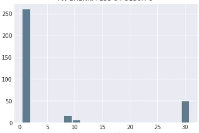
y = array([[ 0.50423378, 0.50423378, 0.50423378, 0.50254455, 0.50423378, 0.50254455, 0.50423378, 0.50507627, 0.50507627, 0.50423378,0.50507627, 0.50507627, 0.50423378, 0.50423378, 0.50423378, 0.50423378, 0.50423378, 0.50423378, 0.50254455, 0.50254455, 0.50254455, 0.50423378, 0.50423378, 0.50507627, 0.50507627,0.50507627, 0.50507627, 0.50507627, 0.50423378, 0.50423378, 0.50423378, 0.50507627, 0.50507627, 0.50423378, 0.50507627, 0.50507627, 0.50507627, 0.50423378, 0.50423378, 0.50423378,0.50423378, 0.50423378, 0.50254455, 0.50254455, 0.5, 0.50254455, 0.50254455, 0.50254455, 0.50423378, 0.50423378,0.50423378, 0.50423378, 0.50423378, 0.50254455, 0.50423378, 0.50254455, 0.50254455, 0.50423378, 0.50423378, 0.50254455,0.5 , 0.5 , 0.50254455, 0.50254455, 0.5 ,0.49658699, 0.49228746, 0.49228746, 0.48707792, 0.48092881,0.48707792, 0.48092881, 0.48092881, 0.48092881, 0.48092881,0.48092881, 0.48092881, 0.47380354, 0.47380354, 0.48092881,0.48707792, 0.48707792, 0.48092881, 0.48092881, 0.48092881,0.48092881, 0.48092881, 0.48092881, 0.47380354, 0.48092881,0.48092881, 0.48092881, 0.48707792, 0.48707792, 0.48707792,0.49228746, 0.49228746, 0.49228746, 0.49228746, 0.48707792,0.48707792, 0.48707792, 0.49228746, 0.48707792, 0.48707792,0.48707792, 0.48707792, 0.48707792, 0.49228746, 0.49228746,0.48707792, 0.48707792, 0.49228746, 0.49658699, 0.49658699,0.49658699, 0.49228746, 0.49228746, 0.49658699, 0.49228746,0.49658699, 0.5 , 0.50254455, 0.50423378, 0.50423378,0.50254455, 0.50423378, 0.50423378, 0.50254455, 0.5 ,0.5 , 0.5 , 0.5 , 0.5 , 0.50254455,0.50254455, 0.5 , 0.50254455, 0.5 , 0.5 ,0.5 , 0.5 , 0.5 , 0.5 , 0.49658699,0.49228746, 0.48707792, 0.48707792, 0.48707792, 0.49228746,0.49228746, 0.48707792, 0.48707792, 0.49228746, 0.48707792,0.48707792, 0.48707792, 0.48092881, 0.48092881, 0.48707792,0.48707792, 0.48092881, 0.47380354, 0.48092881, 0.48092881,0.48707792, 0.49228746, 0.48707792, 0.49228746, 0.48707792,0.48092881, 0.47380354, 0.46565731, 0.46565731, 0.46565731,0.45643546, 0.45643546, 0.45643546, 0.45643546, 0.45643546,0.45643546, 0.45643546, 0.46565731, 0.45643546, 0.45643546,0.45643546, 0.44607129, 0.45643546, 0.45643546, 0.45643546,0.44607129, 0.44607129, 0.43448304, 0.43448304, 0.43448304,0.44607129, 0.45643546, 0.45643546, 0.45643546, 0.46565731,0.47380354, 0.48092881, 0.48092881, 29.38186886, 29.38186886,29.38186886, 29.37898909, 29.45299206, 29.52449116, 29.74083063,29.73771398, 29.73771398, 29.74083063, 29.74083063, 29.74083063,29.74083063, 29.73771398, 29.74083063, 29.73771398, 29.73771398,29.73771398, 29.73771398, 29.74083063, 29.74083063, 29.74083063,30.12527698, 30.48367189, 30.8169243 , 30.8169243 , 30.8169243 ,30.8169243 , 30.82153203, 30.8169243 , 30.81230208, 30.81230208,30.80766536, 30.81230208, 30.81230208, 30.80766536, 30.80301414,30.80301414, 30.80301414, 30.80301414, 30.80301414, 30.80766536,30.81230208, 30.81230208, 30.81230208, 30.81230208, 30.8169243 ,30.82153203, 30.82612528, 10.51949923, 10.51949923, 10.51436497,10.51436497, 10.22456193, 9.91464422, 9.36922158, 9.37416663,9.36922158, 9.36922158, 9.36922158, 9.37416663, 9.37906375,9.383913 , 9.383913 , 9.38871446, 9.383913 , 9.37906375,9.37416663, 9.36922158, 9.36422851, 9.35918734, 7.72711675,5.53121937, 0.5 , 0.50254455, 0.50254455, 0.50254455,0.50254455, 0.50254455, 0.5 , 0.5 , 0.49658699,0.5 , 0.5 , 0.5 , 0.49658699, 0.49658699,0.5 , 0.50254455, 0.50423378, 0.50423378, 0.50423378,0.50507627, 0.50507627, 0.50423378, 0.50423378, 0.50423378,0.50423378, 0.50423378, 0.50254455, 0.50254455, 0.5 ,0.5 , 0.5 , 0.49658699, 0.5 , 0.49658699,0.49658699, 0.49658699, 0.49658699, 0.49658699, 0.49658699,0.49658699, 0.49658699, 0.49228746, 0.48707792, 0.48707792,0.48092881, 0.47380354, 0.47380354, 0.46565731, 0.46565731,0.47380354, 0.46565731, 0.47380354, 0.47380354, 0.47380354, 0.47380354, 0.48092881]])
使用scipy中的这个例子,我如何获取x数组并将其插入以获取系数,然后在我的分布上绘制curve_fit?
import numpy as np
from scipy.optimize import curve_fit
from scipy.special import gamma as gamma

def betafunc(x,a,b,cst):
    return cst*gamma(a+b) * (x**(a-1)) * ((1-x)**(b-1))  / ( gamma(a)*gamma(b) )

x = np.array( [0.1, 0.3, 0.5, 0.7, 0.9, 1.1])
y = np.array( [0.45112234, 0.56934313, 0.3996803 , 0.28982859, 0.19682153, 0.] )

popt2,pcov2 = curve_fit(betafunc,x[:-1],y[:-1],p0=(0.5,1.5,0.5))

print(popt2)
print(pcov2)