理解scipy的反卷积功能

Question

我正在尝试理解 scipy.signal.deconvolve 函数。

从数学角度来看，卷积只是傅里叶空间中的乘法，因此我期望对于两个函数 f 和 g：

Deconvolve(Convolve(f,g) , g) == f

但在 numpy/scipy 中，要么不是这种情况，要么我忽略了重要的一点。虽然 Stack Overflow 上有一些与 deconvolve 相关的问题（如这里和这里），但它们并没有解决这个问题，其他一些问题则不清楚（这里）或者无人回答（这里）。信号处理 SE 上也有两个问题（这里和这里），但它们的答案并不能帮助理解 scipy 的 deconvolve 函数是如何工作的。

问题是：

• 如果你知道卷积函数 g，如何从经过卷积后的信号中重建原始信号 f？
• 换句话说：这个伪代码 Deconvolve(Convolve(f,g) , g) == f 在 numpy/scipy 中如何实现？

编辑：请注意，本问题不针对防止数值误差（尽管这也是一个开放问题），而是针对理解在 scipy 中如何结合使用 convolve/deconvolve。

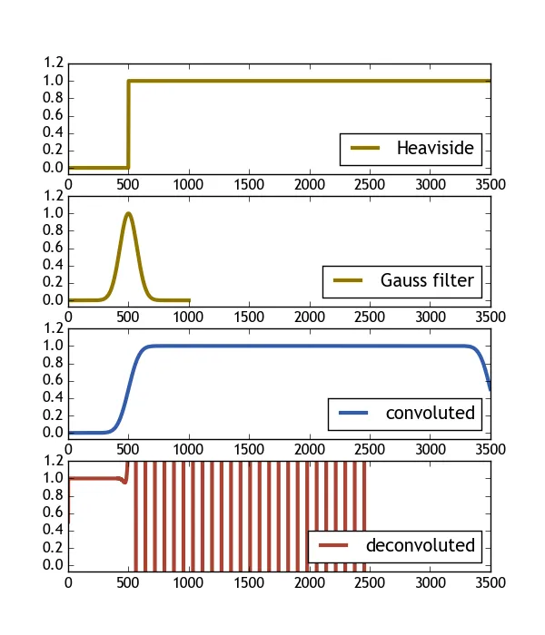
以下代码使用 Heaviside 函数和高斯滤波器来尝试解决这个问题。正如图像中所示，卷积的反卷积结果与原始的 Heaviside 函数完全不同。如果有人能够澄清这个问题，我将不胜感激。

import numpy as np
import scipy.signal
import matplotlib.pyplot as plt

# Define heaviside function
H = lambda x: 0.5 * (np.sign(x) + 1.)
#define gaussian
gauss = lambda x, sig: np.exp(-( x/float(sig))**2 )

X = np.linspace(-5, 30, num=3501)
X2 = np.linspace(-5,5, num=1001)

# convolute a heaviside with a gaussian
H_c = np.convolve( H(X),  gauss(X2, 1),  mode="same"  )
# deconvolute a the result
H_dc, er = scipy.signal.deconvolve(H_c, gauss(X2, 1) )


#### Plot #### 
fig , ax = plt.subplots(nrows=4, figsize=(6,7))
ax[0].plot( H(X),          color="#907700", label="Heaviside",    lw=3 ) 
ax[1].plot( gauss(X2, 1),  color="#907700", label="Gauss filter", lw=3 )
ax[2].plot( H_c/H_c.max(), color="#325cab", label="convoluted" ,  lw=3 ) 
ax[3].plot( H_dc,          color="#ab4232", label="deconvoluted", lw=3 ) 
for i in range(len(ax)):
    ax[i].set_xlim([0, len(X)])
    ax[i].set_ylim([-0.07, 1.2])
    ax[i].legend(loc=4)
plt.show()

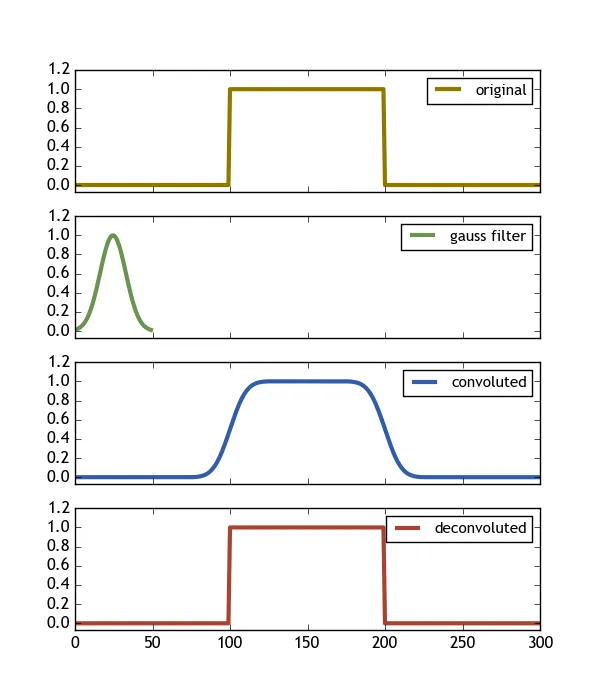
编辑：请注意，这里有一个matlab示例，展示如何使用信号卷积/解卷积一个矩形信号。

yc=conv(y,c,'full')./sum(c); 
ydc=deconv(yc,c).*sum(c); 

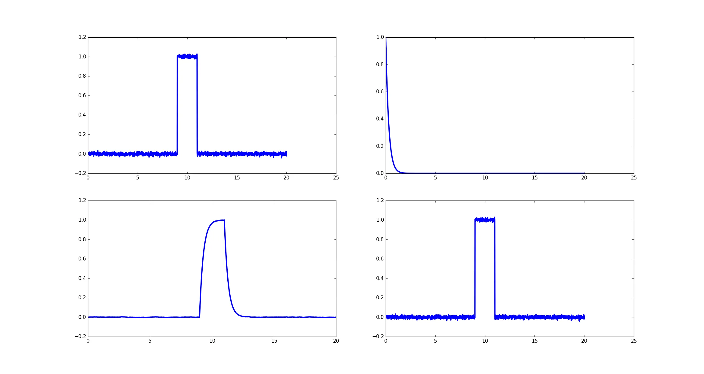
为了回答这个问题，如果有人能够将这个例子翻译成Python，那也会很有帮助。

In the spirit of this question it would also help if someone was able to translate this example into python.

- ImportanceOfBeingErnest

---

使用 mode=full 运行它会得到一个相当不错的结果（直到大约索引1000，然后可能会出现边界效应）；不幸的是，我对这个理论了解得不够。 - Cleb

@Cleb 不错。但是首先使用 mode="full" 运行它会将卷积信号向右移动，使得边缘在这种情况下位于1000而不是500。你有什么想法吗？如何解释卷积数组的结果与原始数组相比？ - ImportanceOfBeingErnest

操作 np.convolve(f,g) 可能是（a）不可逆的，或者（b）它的反演可能在数值上不稳定，这取决于 g。deconvolve 只能成功找到“良好行为”函数g的有限类别中的f。您的问题更适合于信号处理SE。 - Stelios

@ImportanceOfBeingErnest，您在帖子中明确提出了一个问题：“如果您知道卷积函数g，如何从卷积信号中重构原始信号f？”这基于先验假设Deconvolve(Convolve(f,g) , g) == f成立。我只是指出后者通常不成立。 - Stelios

是的，这只是我能够重建它的唯一方式；也许你应该像Stelios建议的那样在信号处理SE上提出这个问题。我想我无法再提供更多帮助了 :( - Cleb

Answer 1

经过一番试验和错误，我发现如何解释scipy.signal.deconvolve()的结果，并将我的发现发布为答案。

让我们从一个可行的代码示例开始。

import numpy as np
import scipy.signal
import matplotlib.pyplot as plt

# let the signal be box-like
signal = np.repeat([0., 1., 0.], 100)
# and use a gaussian filter
# the filter should be shorter than the signal
# the filter should be such that it's much bigger then zero everywhere
gauss = np.exp(-( (np.linspace(0,50)-25.)/float(12))**2 )
print gauss.min()  # = 0.013 >> 0

# calculate the convolution (np.convolve and scipy.signal.convolve identical)
# the keywordargument mode="same" ensures that the convolution spans the same
#   shape as the input array.
#filtered = scipy.signal.convolve(signal, gauss, mode='same') 
filtered = np.convolve(signal, gauss, mode='same') 

deconv,  _ = scipy.signal.deconvolve( filtered, gauss )
#the deconvolution has n = len(signal) - len(gauss) + 1 points
n = len(signal)-len(gauss)+1
# so we need to expand it by 
s = (len(signal)-n)/2
#on both sides.
deconv_res = np.zeros(len(signal))
deconv_res[s:len(signal)-s-1] = deconv
deconv = deconv_res
# now deconv contains the deconvolution 
# expanded to the original shape (filled with zeros) 


#### Plot #### 
fig , ax = plt.subplots(nrows=4, figsize=(6,7))

ax[0].plot(signal,            color="#907700", label="original",     lw=3 ) 
ax[1].plot(gauss,          color="#68934e", label="gauss filter", lw=3 )
# we need to divide by the sum of the filter window to get the convolution normalized to 1
ax[2].plot(filtered/np.sum(gauss), color="#325cab", label="convoluted" ,  lw=3 )
ax[3].plot(deconv,         color="#ab4232", label="deconvoluted", lw=3 ) 

for i in range(len(ax)):
    ax[i].set_xlim([0, len(signal)])
    ax[i].set_ylim([-0.07, 1.2])
    ax[i].legend(loc=1, fontsize=11)
    if i != len(ax)-1 :
        ax[i].set_xticklabels([])

plt.savefig(__file__ + ".png")
plt.show()    

这段代码会生成以下图片，展示了我们所需的东西 (Deconvolve(Convolve(signal,gauss), gauss) == signal)

一些重要的发现包括：

• 滤波器应该比信号短
• 滤波器在每个位置上的数值都应该大于零（这里 > 0.013 就足够好了）
• 使用关键字参数mode = 'same'进行卷积可以确保其与信号具有相同的数组形状。
• 去卷积结果有n = len(signal) - len(gauss) + 1个点。因此，为了让它也与原始数组形状相同，我们需要在两侧扩展s = (len(signal)-n)/2。

当然，对此问题的更多发现、评论和建议仍然受欢迎。

- ImportanceOfBeingErnest

---

你是靠自己找出最佳长度和最小过滤器值的，还是在某些地方找到了相关来源？ - Cleb

@Cleb 我没有找到任何来源，这都是基于试错的。与您对Matlab代码的翻译相比，即使滤波器与信号具有相同的形状，整个过程似乎也可以工作。我认为原因是，滤波器的第一个点需要比零大得多（如果它恰好等于零，甚至会抛出错误）。 - ImportanceOfBeingErnest

好的。也许这个 Matlab 的翻译可以帮到你…… 我会不时关注这个问题，看是否会有更好的答案出现。祝你的项目好运！ - Cleb

是的，确实如此。对于其他寻求此类建议的人来说也可能有帮助。谢谢。 - ImportanceOfBeingErnest

先生们，您在过去两年中是否学到了关于这个主题的新知识？我发现您的例子很有帮助，只是填充似乎过多。我无法相信只能在信号和滤波器完全交叉的点上进行反卷积。简单地说，方程的数量总是与未知数一样多，因此应该可以重建整个信号，而不仅仅是中间部分。也许朝向末尾的值会比中间的不太准确，但仍然如此。有什么想法吗？ - Aleksejs Fomins

Answer 2

正如评论中所写的，我无法帮助你解决最初发布的示例。正如@Stelios指出的那样，由于数值问题，反卷积可能无法正常工作。

但是，我可以重现您在编辑中发布的示例：

这是直接从matlab源代码翻译而来的代码:

import numpy as np
import scipy.signal
import matplotlib.pyplot as plt

x = np.arange(0., 20.01, 0.01)
y = np.zeros(len(x))
y[900:1100] = 1.
y += 0.01 * np.random.randn(len(y))
c = np.exp(-(np.arange(len(y))) / 30.)

yc = scipy.signal.convolve(y, c, mode='full') / c.sum()
ydc, remainder = scipy.signal.deconvolve(yc, c)
ydc *= c.sum()

fig, ax = plt.subplots(nrows=2, ncols=2, figsize=(4, 4))
ax[0][0].plot(x, y, label="original y", lw=3)
ax[0][1].plot(x, c, label="c", lw=3)
ax[1][0].plot(x[0:2000], yc[0:2000], label="yc", lw=3)
ax[1][1].plot(x, ydc, label="recovered y", lw=3)

plt.show()

- Cleb