pykalman:（默认）处理缺失值

Question

我正在使用pykalman模块中的KalmanFilter，并想知道它如何处理缺失观测值。根据文档：

在现实世界的系统中，传感器偶尔会出现故障。卡尔曼滤波器、卡尔曼平滑算法和EM算法都能够处理这种情况。要利用它，只需要在缺失的时间步骤上应用一个NumPy掩码来测量：

from numpy import ma X = ma.array([1,2,3]) X1 = ma.masked # hide measurement at time step 1 kf.em(X).smooth(X)

我们可以平滑输入的时间序列。由于这是一个“附加”函数，我认为它不会自动执行；那么当变量中有NaN时，默认的方法是什么？

这里解释了可能发生的理论方法；这也是pykalman所做的吗（在我看来这将非常棒）：

交叉验证 - 如何处理卡尔曼滤波中的不完整数据？

- eternity1

Answer 1

让我们来看一下源代码：

filter_update函数中，pykalman检查当前观测值是否被掩盖。

def filter_update(...)

        # Make a masked observation if necessary
        if observation is None:
            n_dim_obs = observation_covariance.shape[0]
            observation = np.ma.array(np.zeros(n_dim_obs))
            observation.mask = True
        else:
            observation = np.ma.asarray(observation) 

这不会影响预测步骤。但是校正步骤有两个选项。它发生在_filter_correct函数中。

def _filter_correct(...)

    if not np.any(np.ma.getmask(observation)):

         # the normal Kalman Filter math

    else:
        n_dim_state = predicted_state_covariance.shape[0]
        n_dim_obs = observation_matrix.shape[0]
        kalman_gain = np.zeros((n_dim_state, n_dim_obs))

        # !!!! the corrected state takes the result of the prediction !!!!

        corrected_state_mean = predicted_state_mean
        corrected_state_covariance = predicted_state_covariance

正如您所看到的，这正是理论方法。

这里有一个简短的例子和可用的工作数据。

假设您有一个GPS接收器，并且您想在步行时跟踪自己。接收器具有很高的精度。为简化起见，假设您只向前直走。

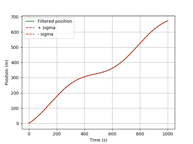
没有什么有趣的事情发生。由于良好的GPS信号，滤波器非常准确地估计了您的位置。如果您有一段时间没有信号会发生什么？

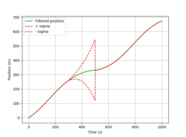
滤波器只能根据现有状态和对系统动态的知识进行预测（请参见矩阵Q）。随着每个预测步骤，不确定性增加。估计位置周围的1-Sigma范围变大。一旦再次出现新的观测，状态就会被纠正。

这是代码和数据：

from pykalman import KalmanFilter
import numpy as np
import matplotlib.pyplot as plt
from numpy import ma

# enable or disable missing observations
use_mask = 1

# reading data (quick and dirty)
Time=[]
X=[]

for line in open('data/dataset_01.csv'):
    f1, f2  = line.split(';')
    Time.append(float(f1))
    X.append(float(f2))

if (use_mask):
    X = ma.asarray(X)
    X[300:500] = ma.masked

# Filter Configuration

# time step
dt = Time[2] - Time[1]

# transition_matrix  
F = [[1,  dt,   0.5*dt*dt], 
     [0,   1,          dt],
     [0,   0,           1]]  

# observation_matrix   
H = [1, 0, 0]

# transition_covariance 
Q = [[   1,     0,     0], 
     [   0,  1e-4,     0],
     [   0,     0,  1e-6]] 

# observation_covariance 
R = [0.04] # max error = 0.6m

# initial_state_mean
X0 = [0,
      0,
      0]

# initial_state_covariance
P0 = [[ 10,    0,   0], 
      [  0,    1,   0],
      [  0,    0,   1]]

n_timesteps = len(Time)
n_dim_state = 3

filtered_state_means = np.zeros((n_timesteps, n_dim_state))
filtered_state_covariances = np.zeros((n_timesteps, n_dim_state, n_dim_state))

# Kalman-Filter initialization
kf = KalmanFilter(transition_matrices = F, 
                  observation_matrices = H, 
                  transition_covariance = Q, 
                  observation_covariance = R, 
                  initial_state_mean = X0, 
                  initial_state_covariance = P0)


# iterative estimation for each new measurement
for t in range(n_timesteps):
    if t == 0:
        filtered_state_means[t] = X0
        filtered_state_covariances[t] = P0
    else:
        filtered_state_means[t], filtered_state_covariances[t] = (
        kf.filter_update(
            filtered_state_means[t-1],
            filtered_state_covariances[t-1],
            observation = X[t])
        )

position_sigma = np.sqrt(filtered_state_covariances[:, 0, 0]);        

# plot of the resulted trajectory        
plt.plot(Time, filtered_state_means[:, 0], "g-", label="Filtered position", markersize=1)
plt.plot(Time, filtered_state_means[:, 0] + position_sigma, "r--", label="+ sigma", markersize=1)
plt.plot(Time, filtered_state_means[:, 0] - position_sigma, "r--", label="- sigma", markersize=1)
plt.grid()
plt.legend(loc="upper left")
plt.xlabel("Time (s)")
plt.ylabel("Position (m)")
plt.show()      

更新

如果你遮盖一个更长的时间段（300:700），这个问题看起来更有趣。

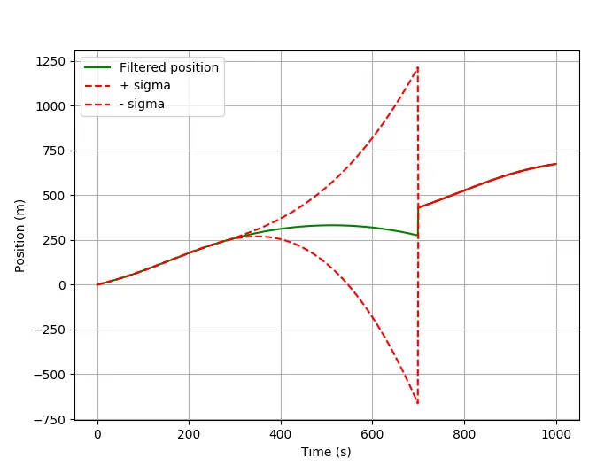
正如你所看到的，位置会回退。这是由于转移矩阵 F 的影响，该矩阵将位置、速度和加速度的预测值绑定在一起。

如果您查看速度状态，则可以解释位置的下降。

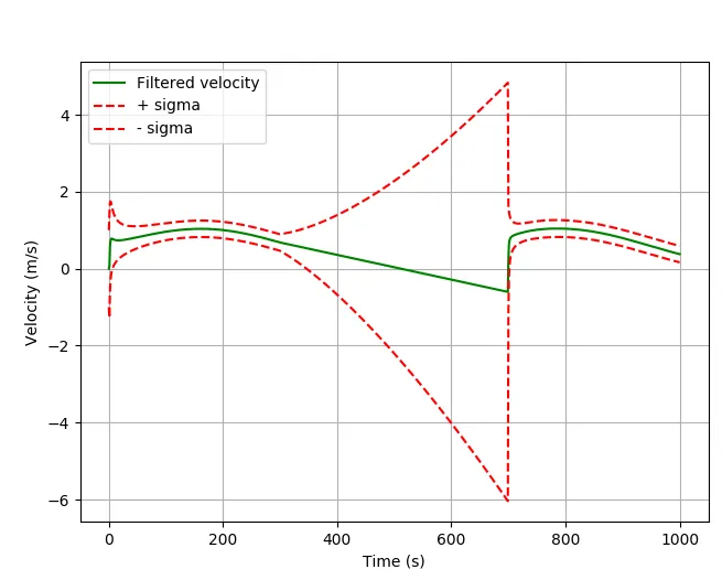
在 300 秒的时间点上，加速度冻结。速度以恒定的斜率下降并穿过 0 值。此时间点之后，位置必须返回。

要绘制速度，请使用以下代码：

velocity_sigma = np.sqrt(filtered_state_covariances[:, 1, 1]);     

# plot of the estimated velocity        
plt.plot(Time, filtered_state_means[:, 1], "g-", label="Filtered velocity", markersize=1)
plt.plot(Time, filtered_state_means[:, 1] + velocity_sigma, "r--", label="+ sigma", markersize=1)
plt.plot(Time, filtered_state_means[:, 1] - velocity_sigma, "r--", label="- sigma", markersize=1)
plt.grid()
plt.legend(loc="upper left")
plt.xlabel("Time (s)")
plt.ylabel("Velocity (m/s)")
plt.show()   

- Anton