非参数分位数回归曲线用于散点图。

Question

我创建了一个散点图（多组GRP），其中IV=time，DV=concentration。 我想在我的图中添加分位数回归曲线(0.025,0.05,0.5,0.95,0.975)。

顺便说一下，这是我创建散点图的方法：

attach(E)  ## E is the name I gave to my data
## Change Group to factor so that may work with levels in the legend
Group<-as.character(Group)
Group<-as.factor(Group)

## Make the colored scatter-plot
mycolors = c('red','orange','green','cornflowerblue')
plot(Time,Concentration,main="Template",xlab="Time",ylab="Concentration",pch=18,col=mycolors[Group])

## This also works identically
## with(E,plot(Time,Concentration,col=mycolors[Group],main="Template",xlab="Time",ylab="Concentration",pch=18))

## Use identify to identify each point by group number (to check)
## identify(Time,Concentration,col=mycolors[Group],labels=Group)
## Press Esc or press Stop to stop identify function

## Create legend
## Use locator(n=1,type="o") to find the point to align top left of legend box
legend('topright',legend=levels(Group),col=mycolors,pch=18,title='Group')

因为我在这里创建的数据是我更大数据集的一个小子集，所以它看起来可以近似为一个矩形双曲线。但我不想现在就称呼我的自变量和因变量之间的数学关系。

我认为来自quantreg包的nlrq可能是答案，但我不知道如何在不知道变量之间关系的情况下使用该函数。

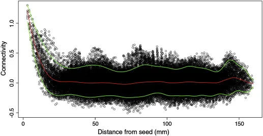
我从一篇科学文章中找到了这张图，并且我想做完全相同类型的图表： 再次感谢您的帮助！

更新 Test.csv 有人指出我的样本数据无法再现。这是我的一些数据样本。

library(evd)
qcbvnonpar(p=c(0.025,0.05,0.5,0.95,0.975),cbind(TAD,DV),epmar=T,plot=F,add=T)

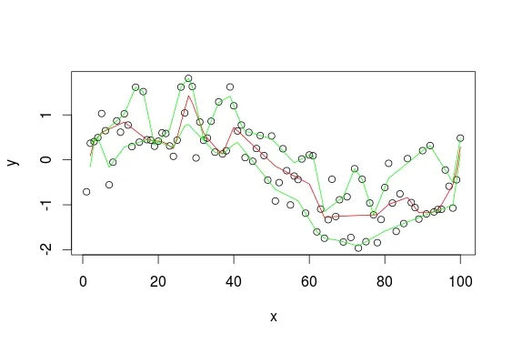
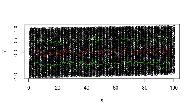
我也尝试了qcbvnonpar::evd，但曲线似乎不太平滑。

- shirleywu

---

如果您无法提供自己的数据，请尝试创建一个随机数数据集并演示您的问题。展示您所尝试的方法，这样不仅让我们有了具体的可操作性，而且也是一种诚信的表现。 - sebastian-c

哦，对不起——我会编造一些数字。可能会相当大。 - shirleywu

这可能有助于您生成数据。https://dev59.com/eG025IYBdhLWcg3whGSx - Roman Luštrik

也许 quantreg 中的 rqss() 适合您？ - EDi

@Roman Luštrik：我会保存这个页面以备将来参考。看起来我的问题在较小的数据集上无法重现，我想我看到有人发布了一个大文件的dropbox链接，将来我也可能会这样做。 - shirleywu

Answer 1

也许您可以查看quantreg:::rqss，以平滑样条和分位数回归。 对于不太好的示例数据，我感到抱歉：

set.seed(1234)
period <- 100
x <- 1:100
y <- sin(2*pi*x/period) + runif(length(x),-1,1)


require(quantreg)
mod <- rqss(y ~ qss(x))
mod2 <- rqss(y ~ qss(x), tau=0.75)
mod3 <- rqss(y ~ qss(x), tau=0.25)
plot(x, y)
lines(x[-1], mod$coef[1] + mod$coef[-1], col = 'red')
lines(x[-1], mod2$coef[1] + mod2$coef[-1], col = 'green')
lines(x[-1], mod3$coef[1] + mod3$coef[-1], col = 'green')

- EDi

---

如果需要非参数化，且示例图像表明它是基于样条的拟合，则对于rqss()函数我肯定会首先考虑。 - Gavin Simpson

它在你的示例中运行得如此完美，但我不确定为什么，即使我检查了我的x和y具有相同的n，但对于我的数据集，我仍然会收到“xy.coords（x，y）中的错误：'x'和'y'长度不同”的警告。仍在努力调试错误 :P - shirleywu

你能给我们更多的数据吗？你上面的示例数据显然不太合适。 - EDi

Answer 2

过去，我经常在使用rqss时遇到困难，而我的问题几乎总是与点的排序有关。

你需要在不同的时间点进行多次测量，这就是为什么你得到不同长度的原因。以下方法适用于我：

dat <- read.csv("~/Downloads/Test.csv")

library(quantreg)
dat <- plyr::arrange(dat,Time)
fit<-rqss(Concentration~qss(Time,constraint="N"),tau=0.5,data = dat)
with(dat,plot(Time,Concentration))
lines(unique(dat$Time)[-1],fit$coef[1] + fit$coef[-1])

对于拟合模型来说，在进行之前优先对数据框进行排序似乎是必要的。

- joran

---

这个可行！非常感谢。我不知道排序可能是一个问题。 - shirleywu

Answer 3

如果您想要使用 ggplot2 绘制图形...

我基于 @EDi 的示例进行了修改。我增加了 x 和 y 的值，以使分位数线更加平滑。由于这种增加，我需要在某些调用中使用 unique(x) 替换 x。

以下是修改后的设置:

set.seed(1234)
period <- 100
x <- rep(1:100,each=100)
y <- 1*sin(2*pi*x/period) + runif(length(x),-1,1)


require(quantreg)
mod <- rqss(y ~ qss(x))
mod2 <- rqss(y ~ qss(x), tau=0.75)
mod3 <- rqss(y ~ qss(x), tau=0.25)

这里有两个图表：

# @EDi's base graphics example
plot(x, y)
lines(unique(x)[-1], mod$coef[1] + mod$coef[-1], col = 'red')
lines(unique(x)[-1], mod2$coef[1] + mod2$coef[-1], col = 'green')
lines(unique(x)[-1], mod3$coef[1] + mod3$coef[-1], col = 'green')

# @swihart's ggplot2 example:
## get into dataset so that ggplot2 can have some fun:
qrdf <- data.table(x       = unique(x)[-1],
                   median =  mod$coef[1] +  mod$coef[-1],
                   qupp   = mod2$coef[1] + mod2$coef[-1],
                   qlow   = mod3$coef[1] + mod3$coef[-1]
)

line_size = 2
ggplot() +
  geom_point(aes(x=x, y=y),
             color="black", alpha=0.5) +
  ## quantiles:
  geom_line(data=qrdf,aes(x=x, y=median),
            color="red", alpha=0.7, size=line_size) +
  geom_line(data=qrdf,aes(x=x, y=qupp),
            color="blue", alpha=0.7, size=line_size, lty=1) +
  geom_line(data=qrdf,aes(x=x, y=qlow),
            color="blue", alpha=0.7, size=line_size, lty=1) 

- swihart