梯度下降似乎失败了

Question

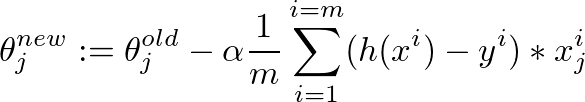
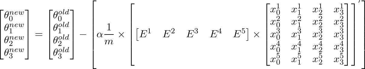
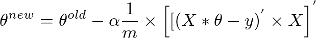
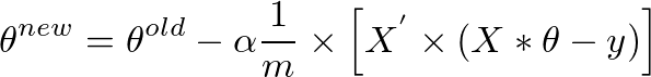
我使用梯度下降算法实现了一个代价函数，以获得一种假设来判断图像的质量。我是用Octave完成的。这个想法在某种程度上基于Andrew Ng的机器学习课程中的算法。

因此，我有880个值为0.5到~12的"y"值。我有880个值为50到300的"X"值，应该预测图像的质量。

不幸的是，算法似乎失败了，经过一些迭代后，theta的值变得非常小，theta0和theta1变成了"NaN"。我的线性回归曲线有奇怪的值...

以下是梯度下降算法的代码： (theta = zeros(2, 1);, alpha= 0.01, iterations=1500)

function [theta, J_history] = gradientDescent(X, y, theta, alpha, num_iters)

m = length(y); % number of training examples
J_history = zeros(num_iters, 1);

for iter = 1:num_iters


    tmp_j1=0;
for i=1:m, 
    tmp_j1 = tmp_j1+ ((theta (1,1) + theta (2,1)*X(i,2)) - y(i));
end

    tmp_j2=0;
for i=1:m, 
    tmp_j2 = tmp_j2+ (((theta (1,1) + theta (2,1)*X(i,2)) - y(i)) *X(i,2)); 
end

    tmp1= theta(1,1) - (alpha *  ((1/m) * tmp_j1))  
    tmp2= theta(2,1) - (alpha *  ((1/m) * tmp_j2))  

    theta(1,1)=tmp1
    theta(2,1)=tmp2

    % ============================================================

    % Save the cost J in every iteration    
    J_history(iter) = computeCost(X, y, theta);
end
end

这里是成本函数的计算：

function J = computeCost(X, y, theta)   %

m = length(y); % number of training examples
J = 0;
tmp=0;
for i=1:m, 
    tmp = tmp+ (theta (1,1) + theta (2,1)*X(i,2) - y(i))^2; %differenzberechnung
end
J= (1/(2*m)) * tmp
end

- Tyzak

---

我猜你跳过了矢量化讲座-就像我一样 ;) https://class.coursera.org/ml-007/lecture/30 - HaveAGuess

Answer 1

如果您想知道看起来很复杂的for循环如何被向量化并压缩成单行表达式，请继续阅读。向量化形式为： theta = theta - (alpha/m) * (X' * (X * theta - y)) 以下是我们使用梯度下降算法得出这个向量化表达式的详细说明：

这是用于微调θ值的梯度下降算法： 假设给定了X、y和θ的以下值：

- m=训练样例数 - n=特征数+1

这里是：

• m = 5（训练样本）
• n = 4（特征+1）
• X = m x n 矩阵
• y = m x 1 向量矩阵
• θ = n x 1 向量矩阵
• xⁱ 是第i个训练样本
• x_j 是给定训练样本中的第j个特征

此外，

• h(x) = ([X] * [θ])（m x 1 预测值矩阵）
• h(x)-y = ([X] * [θ] - [y])（m x 1 预测误差矩阵）

机器学习的整个目标是最小化预测误差。基于上述推论，我们的误差矩阵是一个 m x 1 向量矩阵，如下所示：

为了计算 θ_j 的新值，我们需要将所有误差（m 行）与训练集 X 的第 j 个特征值相乘并求和。也就是说，将 E 中的所有值分别与相应的训练示例的第 j 个特征相乘，并将它们全部加起来。这将有助于我们获得新的（希望更好的）θ_j 值。对所有 j 或特征数量重复此过程。在矩阵形式下，这可以写成：

这可以简化为：

• [E]' x [X]将给我们一个行向量矩阵，因为E'是1 x m矩阵，而X是m x n矩阵。但我们有兴趣得到一个列矩阵，因此我们转置结果矩阵。

更简洁地说，它可以写成： 由于(A * B)' = (B' * A')，并且A'' = A，我们也可以将上述内容写成

这是我们最初开始使用的原始表达式：

theta = theta - (alpha/m) * (X' * (X * theta - y))

- jerrymouse

---

这太有帮助了——矩阵数学的冗长描述对我来说大有裨益。 - rbellamy

Answer 2

我向量化了theta的东西...可能会帮助某些人

theta = theta - (alpha/m *  (X * theta-y)' * X)';

- Markus

---

这个是正确答案。另一种写法是：theta = theta - alpha / m * (X' * (X * theta - y)); 尽可能使用向量化。 - Xiao Hanyu

啊，太好了，我知道一定有方法的，但是我在纸面计算上算不对 ;) - HaveAGuess

对于那些复制粘贴的人：这只是针对线性激活函数的正确更新，而不是对于Sigmoid和其他所有东西。 - davidhigh

为什么不是这样的：theta = theta - (alpha/m) * sum(((X * theta) - y)' * X);？梯度下降方程包含一个求和。 - SalmaFG

你只想对每个theta的值进行求和，而不是所有theta的结果。X' * (x * theta -y) 最终需要得到一个1X2向量。使用sum函数会导致一个1X1向量，这会破坏矩阵代数。 - user249806

在下面写了一个详细的答案来解释为什么Markus的答案是正确的 https://dev59.com/tmkv5IYBdhLWcg3wnB87#42330833 - jerrymouse

Answer 3

我认为你的computeCost函数有误。我去年参加了NG的课程，以下是我的实现（向量化）：

m = length(y);
J = 0;
predictions = X * theta;
sqrErrors = (predictions-y).^2;

J = 1/(2*m) * sum(sqrErrors);

我认为其余的实现看起来都很好，尽管你也可以将它们向量化。

theta_1 = theta(1) - alpha * (1/m) * sum((X*theta-y).*X(:,1));
theta_2 = theta(2) - alpha * (1/m) * sum((X*theta-y).*X(:,2));

随后，您正在将临时theta（这里称为theta_1和theta_2）正确设置回“真实”theta。

通常，向量化而不是循环更有用，阅读和调试更少烦人。

- Thomas Jungblut

---

我去年也参加了这门课程，现在想将解决方案映射到一个当前的问题上；），所以你的答案应该没问题；)) - Tyzak

顺便说一句，也许我忘了，但第一个不应该是吗？ theta_1 = theta(1) - alpha * (1/m) * sum(X*theta - y) - Sumit Nigam

谢谢，我使用了循环而不是向量化，遇到了同样的问题，真是救命稻草！同意，看起来更聪明。 - HaveAGuess

向量化形式也可在多个特征之间进行扩展。 - Edwin O.

Answer 4

如果您可以使用最小二乘代价函数，那么您可以尝试使用正规方程而不是梯度下降。它更简单 - 只有一行代码 - 并且计算速度更快。

这是正规方程： http://mathworld.wolfram.com/NormalEquation.html 在Octave中的表现形式：

theta = (pinv(X' * X )) * X' * y

这是一篇教程，说明如何使用正规方程求解线性回归问题：http://www.lauradhamilton.com/tutorial-linear-regression-with-octave

- user2437742

---

问题涉及梯度下降。 正规方程也可以使用。 - naren

Answer 5

虽然循环计算的梯度下降法不如向量化版本具有可扩展性，但应该会产生相同的结果。在上面的示例中，梯度下降未能计算正确的theta的最可能情况是alpha的值。

使用经过验证的成本和梯度下降函数以及与问题描述中类似的数据集，如果将alpha设置为0.01，则theta在几次迭代后就会出现NaN值。然而，当将其设置为0.000001时，即使经过100次迭代，梯度下降也能按预期工作。

- AdiGri

Answer 6

这样更清晰，也更向量化

predictions = X * theta;
errorsVector = predictions - y;
theta = theta - (alpha/m) * (X' * errorsVector);

- Edwin O.

Answer 7

这应该能够工作：-

theta(1,1) = theta(1,1) - (alpha*(1/m))*((X*theta - y)'* X(:,1) ); 

theta(2,1) = theta(2,1) - (alpha*(1/m))*((X*theta - y)'* X(:,2) ); 

- Gator-aid

Answer 8

仅使用向量，以下是在Mathematica中使用梯度下降实现LR的紧凑代码：

Theta = {0, 0}
alpha = 0.0001;
iteration = 1500;
Jhist = Table[0, {i, iteration}];
Table[  
  Theta = Theta - 
  alpha * Dot[Transpose[X], (Dot[X, Theta] - Y)]/m; 
  Jhist[[k]] = 
  Total[ (Dot[X, Theta] - Y[[All]])^2]/(2*m); Theta, {k, iteration}]

注意：当然，人们假设X是一个n * 2的矩阵，其中X [[，1]]仅包含1。

- user34018

Answer 9

如果您还记得机器学习课程中梯度下降的第一个PDF文件，您会注意到学习率的重要性。这是来自上述PDF的说明。

实现说明：如果您的学习率过大，则J(theta)可能会发散并失控'，导致计算机计算出的值太大。在这种情况下，Octave / MATLAB往往会返回NaNs。 NaN代表不是数字'，通常由涉及-无穷大和+无穷大的未定义操作引起。

- morteza