梯度下降Matlab实现

Question

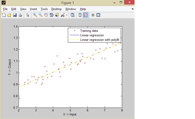
我已经查看了许多stackoverflow上的代码，并在同一行上编写了自己的代码。但是存在一些问题，我无法理解。为了分析目的，我正在存储theta1和theta2的值以及成本函数。可以从这个Openclassroom页面下载x和Y数据，它们以.dat文件的形式提供，您可以在记事本中打开。

    %Single Variate Gradient Descent Algorithm%%
    clc
clear all
close all;
% Step 1 Load x series/ Input data and Output data* y series

x=load('D:\Office Docs_Jay\software\ex2x.dat');
y=load('D:\Office Docs_Jay\software\ex2y.dat');
%Plot the input vectors
plot(x,y,'o');
ylabel('Height in meters');
xlabel('Age in years');

% Step 2 Add an extra column of ones in input vector
[m n]=size(x);
X=[ones(m,1) x];%Concatenate the ones column with x;
% Step 3 Create Theta vector
theta=zeros(n+1,1);%theta 0,1
% Create temporary values for storing summation

temp1=0;
temp2=0;
% Define Learning Rate alpha and Max Iterations

alpha=0.07;
max_iterations=1;
      % Step 4 Iterate over loop
      for i=1:1:max_iterations

     %Calculate Hypothesis for all training example
     for k=1:1:m
        h(k)=theta(1,1)+theta(2,1)*X(k,2); %#ok<AGROW>
        temp1=temp1+(h(k)-y(k));
        temp2=temp2+(h(k)-y(k))*X(k,2);
     end
     % Simultaneous Update
      tmp1=theta(1,1)-(alpha*1/(2*m)*temp1);
      tmp2=theta(2,1)-(alpha*(1/(2*m))*temp2);
      theta(1,1)=tmp1;
      theta(2,1)=tmp2;
      theta1_history(i)=theta(2,1); %#ok<AGROW>
      theta0_history(i)=theta(1,1); %#ok<AGROW>
      % Step 5 Calculate cost function
      tmp3=0;
      tmp4=0;
      for p=1:m
        tmp3=tmp3+theta(1,1)+theta(2,1)*X(p,1);
        tmp4=tmp4+theta(1,1)+theta(2,1)*X(p,2);
      end
      J1_theta0(i)=tmp3*(1/(2*m)); %#ok<AGROW>
      J2_theta1(i)=tmp4*(1/(2*m)); %#ok<AGROW>


      end
      theta
      hold on;
      plot(X(:,2),theta(1,1)+theta(2,1)*X);

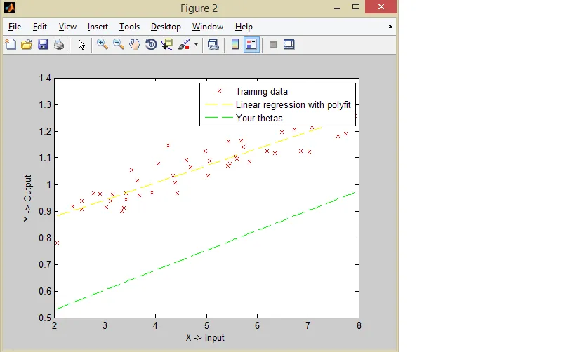
我正在获取值为theta的内容。

在0.0373和0.1900时，它应该是0.0745和0.3800。

这个值大约是我期望值的两倍。

- Incpetor

---

我们没有数据，无法复现您的问题。 - Daniel

嘿，谢谢回复。我已经添加了输入数据链接的链接。 - Incpetor

你好，你必须使用矩阵的属性。这个页面上的答案https://dev59.com/lHzaa4cB1Zd3GeqPRIne#33215224非常优秀。 - Florian Courtial

Answer 1

我一直在尝试使用矩阵和向量完成迭代步骤（即不更新theta的每个参数）。 以下是我想到的（只有梯度步骤在此）:

h = X * theta;  # hypothesis
err = h - y;    # error
gradient = alpha * (1 / m) * (X' * err); # update the gradient
theta = theta - gradient;

难以理解的是，在前面例子中梯度步骤中的“sum”实际上是由矩阵乘法X'*err执行的。

你也可以将其写成(err'*X)'

- cmantas

---

我们也可以写成 sum(X .* err, 1)'，它可以工作（但不够美观）。 - Florian Courtial

感谢cmantas澄清了矩阵乘法的问题，这就是我在编写代码时卡住的地方。我本来打算按照@FlorianCourtial所说的去做，但现在我已经理解得很好了。 - M090009

你能否解释一下为什么 X' * err 也可以作为求和步骤呢？我知道它可以工作，但是我还不太明白它为什么可以这样做。 - yasgur99

我写这篇文章已经有一段时间了，我可能记得不太准确（如果 h 或 err 中的任何一个是向量，请停止读取）。 X 是输入向量的矩阵。对于 n 个数据点和 m 个特征，它是一个 n x m 的矩阵，而 err 是一个大小为 n 的向量（即一个 n x 1 的矩阵）。 因此，X'*err 是 (m x n) * (n x 1) 的矩阵乘法，因此无论 n 多大，其大小始终为 m x 1。 在 矩阵乘法 中，结果的元素 (AB)ij 是通过在中间维度上进行求和获得的-在本例中为 n。请参见 (AB)ij 的公式。 - cmantas

Answer 2

我成功地创建了一个算法，它使用了Matlab支持的更多矢量化属性。我的算法与你的略有不同，但可以执行你要求的梯度下降过程。在我执行和验证（使用polyfit函数）之后，我认为openclassroom（练习2）中期望的theta（0）= 0.0745和theta（1）= 0.3800变量的值在1500次迭代后步长为0.07时是错误的（我没有回应这个问题）。这就是我将我的结果与数据在一个图中绘制并将你需要的结果与数据在另一个图中绘制的原因，并且我看到数据拟合过程存在很大差异。

首先，请查看代码：

% Machine Learning : Linear Regression

clear all; close all; clc;

%% ======================= Plotting Training Data =======================
fprintf('Plotting Data ...\n')

x = load('ex2x.dat');
y = load('ex2y.dat');

% Plot Data
plot(x,y,'rx');
xlabel('X -> Input') % x-axis label
ylabel('Y -> Output') % y-axis label

%% =================== Initialize Linear regression parameters ===================
 m = length(y); % number of training examples

% initialize fitting parameters - all zeros
theta=zeros(2,1);%theta 0,1

% Some gradient descent settings
iterations = 1500;
Learning_step_a = 0.07; % step parameter

%% =================== Gradient descent ===================

fprintf('Running Gradient Descent ...\n')

%Compute Gradient descent

% Initialize Objective Function History
J_history = zeros(iterations, 1);

m = length(y); % number of training examples

% run gradient descent    
for iter = 1:iterations

   % In every iteration calculate hypothesis
   hypothesis=theta(1).*x+theta(2);

   % Update theta variables
   temp0=theta(1) - Learning_step_a * (1/m)* sum((hypothesis-y).* x);
   temp1=theta(2) - Learning_step_a * (1/m) *sum(hypothesis-y);

   theta(1)=temp0;
   theta(2)=temp1;

   % Save objective function 
   J_history(iter)=(1/2*m)*sum(( hypothesis-y ).^2);

end

% print theta to screen
fprintf('Theta found by gradient descent: %f %f\n',theta(1),  theta(2));
fprintf('Minimum of objective function is %f \n',J_history(iterations));

% Plot the linear fit
hold on; % keep previous plot visible 
plot(x, theta(1)*x+theta(2), '-')

% Validate with polyfit fnc
poly_theta = polyfit(x,y,1);
plot(x, poly_theta(1)*x+poly_theta(2), 'y--');
legend('Training data', 'Linear regression','Linear regression with polyfit')
hold off 

figure
% Plot Data
plot(x,y,'rx');
xlabel('X -> Input') % x-axis label
ylabel('Y -> Output') % y-axis label

hold on; % keep previous plot visible
% Validate with polyfit fnc
poly_theta = polyfit(x,y,1);
plot(x, poly_theta(1)*x+poly_theta(2), 'y--');

% for theta values that you are saying
theta(1)=0.0745;  theta(2)=0.3800;
plot(x, theta(1)*x+theta(2), 'g--')
legend('Training data', 'Linear regression with polyfit','Your thetas')
hold off 

好的，结果如下：

通过我的算法得到的theta(0)和theta(1)使得该直线适合这些数据。

当theta(0)和theta(1)固定时，该直线不适合这些数据。

- Konstantinos Monachopoulos

---

这样正确吗：hypothesis=theta(1).*x+theta(2)； 也许你应该像这样修正它> hypothesis=theta(1)+theta(2).*x； - Ivan T

@monakons 如何从CSV文件中加载数据，而不是dat文件，例如：ex2x.csv。 - Eka

dir_of_csv = sprintf('CSV文件所在的目录'); list_of_csv = dir( fullfile(dir_of_csv ,'*.csv') ); list_of_csv_names = {list_of_csv.name}'; - Konstantinos Monachopoulos

Answer 3

从您的期望值和程序结果的 Ɵ（theta）值中可以注意到一件事情，即期望值是结果的两倍。

您可能犯的错误是在导数计算代码中使用了 1/(2*m) 代替 1/m。在导数中，分母的 2 消失了，因为原始项是 (h_Ɵ(x) - y)²，它在微分时生成 2*(h_Ɵ(x) - y)。这两个2会相互抵消。

请修改以下代码行：

J1_theta0(i)=tmp3*(1/(2*m)); %#ok<AGROW>
J2_theta1(i)=tmp4*(1/(2*m)); %#ok<AGROW>

到

J1_theta0(i)=tmp3*(1/m); %#ok<AGROW>
J2_theta1(i)=tmp4*(1/m); %#ok<AGROW>

希望这能有所帮助。

- Arumoy Chakraborty

Answer 4

你需要在迭代循环的第一个注释中放置 temp1=0 temp2=0； 因为如果不这样做，当前的temp将会影响下一次迭代，那是错误的。

- navid

Answer 5

以下是一些评论：

1. max_iterations 被设置为 1。通常会执行梯度下降，直到目标函数的减少在某个阈值以下或者梯度的大小在某个阈值以下，这可能需要多于一次迭代。

2. 1/(2*m) 的因子不是技术上正确的。这不会导致算法失败，但会有效地降低学习速率。

3. 您没有计算正确的目标。正确的线性回归目标应该是平均平方残差的一半，或者是平方残差的总和的一半。

4. 与其使用 for 循环，您应该利用 matlab 的向量化计算。例如，res=X*theta-y; obj=.5/m*res'res; 应该计算出残差 (res) 和线性回归目标 (obj)。

- user1149913

---

感谢您的回复。迭代次数故意保持为1，仅用于测试。当iter=1时，期望的结果是0.0745和0.3800。请参考我在问题中提供的链接。我删除了1/(2*m)部分，得到了不想要的结果。很抱歉，我不明白在我的代码中应该在哪里进行更改。 - Incpetor