梯度下降 Python 实现 - 等高线

Question

作为自学练习，我正在尝试从头开始实现梯度下降算法解决线性回归问题，并在等高线图上绘制结果迭代过程。

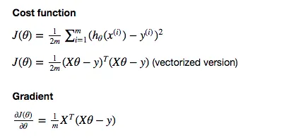
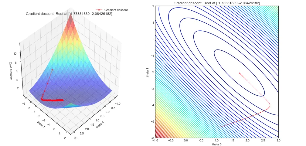
我的梯度下降实现给出了正确的结果（已通过Sklearn测试），但是梯度下降图似乎不与等高线垂直。这是预期的还是我的代码/理解有误？

算法：

成本函数和梯度下降。

import numpy as np
import pandas as pd
from matplotlib import pyplot as plt
from mpl_toolkits.mplot3d import Axes3D

def costfunction(X,y,theta):
    m = np.size(y)

    #Cost function in vectorized form
    h = X @ theta
    J = float((1./(2*m)) * (h - y).T @ (h - y));    
    return J;


def gradient_descent(X,y,theta,alpha = 0.0005,num_iters=1000):
    #Initialisation of useful values 
    m = np.size(y)
    J_history = np.zeros(num_iters)
    theta_0_hist, theta_1_hist = [], [] #For plotting afterwards

    for i in range(num_iters):
        #Grad function in vectorized form
        h = X @ theta
        theta = theta - alpha * (1/m)* (X.T @ (h-y))

        #Cost and intermediate values for each iteration
        J_history[i] = costfunction(X,y,theta)
        theta_0_hist.append(theta[0,0])
        theta_1_hist.append(theta[1,0])

    return theta,J_history, theta_0_hist, theta_1_hist

情节

#Creating the dataset (as previously)
x = np.linspace(0,1,40)
noise = 1*np.random.uniform(  size = 40)
y = np.sin(x * 1.5 * np.pi ) 
y_noise = (y + noise).reshape(-1,1)
X = np.vstack((np.ones(len(x)),x)).T


#Setup of meshgrid of theta values
T0, T1 = np.meshgrid(np.linspace(-1,3,100),np.linspace(-6,2,100))

#Computing the cost function for each theta combination
zs = np.array(  [costfunction(X, y_noise.reshape(-1,1),np.array([t0,t1]).reshape(-1,1)) 
                     for t0, t1 in zip(np.ravel(T0), np.ravel(T1)) ] )
#Reshaping the cost values    
Z = zs.reshape(T0.shape)


#Computing the gradient descent
theta_result,J_history, theta_0, theta_1 = gradient_descent(X,y_noise,np.array([0,-6]).reshape(-1,1),alpha = 0.3,num_iters=1000)

#Angles needed for quiver plot
anglesx = np.array(theta_0)[1:] - np.array(theta_0)[:-1]
anglesy = np.array(theta_1)[1:] - np.array(theta_1)[:-1]

%matplotlib inline
fig = plt.figure(figsize = (16,8))

#Surface plot
ax = fig.add_subplot(1, 2, 1, projection='3d')
ax.plot_surface(T0, T1, Z, rstride = 5, cstride = 5, cmap = 'jet', alpha=0.5)
ax.plot(theta_0,theta_1,J_history, marker = '*', color = 'r', alpha = .4, label = 'Gradient descent')

ax.set_xlabel('theta 0')
ax.set_ylabel('theta 1')
ax.set_zlabel('Cost function')
ax.set_title('Gradient descent: Root at {}'.format(theta_result.ravel()))
ax.view_init(45, 45)


#Contour plot
ax = fig.add_subplot(1, 2, 2)
ax.contour(T0, T1, Z, 70, cmap = 'jet')
ax.quiver(theta_0[:-1], theta_1[:-1], anglesx, anglesy, scale_units = 'xy', angles = 'xy', scale = 1, color = 'r', alpha = .9)

plt.show()

表面和轮廓图

评论

我的理解是，梯度下降法垂直地沿着等高线进行。这不是这样吗？谢谢。

- Xavier Bourret Sicotte

---

梯度下降中的每一步都会减少总拟合误差，这是正确的，但不能保证直接朝向最小值。考虑你在山上螺旋下降的情况 - 每一步都会让你往下走，但不是笔直向下。如果误差空间是“崎岖”的，那么梯度下降也可能会陷入局部误差空间最小值，也就是说，梯度下降中的步骤是朝着更低的误差方向前进，但不一定是朝着最低的误差方向。 - James Phillips

说的不错，但是这个函数是平滑和二次的，没有颠簸和局部极小值... - Xavier Bourret Sicotte

你是正确的，每一步都会减少误差，但方向并不总是直接朝向最小值，而是朝着更低的误差。因此存在“下降”，但不总是沿着直线方向。 - James Phillips

同意，我的问题更在于为什么下降方向与等高线不垂直。它与等高线呈角度关系。 - Xavier Bourret Sicotte

针对总误差的梯度是针对每个参数单独确定的，但在每一步中，所有参数都同时而非单独地改变。这种组合变化可能不垂直于等高线，正如您在此处所看到的。 - James Phillips

Answer 1

等高线图的问题在于theta0和theta1的刻度不同。只需在等高线绘图指令中添加“plt.axis('equal')”，您将看到梯度下降实际上是垂直于等高线。

在两个轴上具有相同刻度的等高线图

- rinicro

Answer 2

通常情况下，梯度下降不遵循等高线。

只有当梯度向量的分量完全相同（绝对值相等）时，才会沿着等高线移动，这意味着在评估点处函数的陡峭程度在每个维度上都相同。

因此，在您的情况下，只有当等高线图中的曲线是同心圆而不是椭圆时才成立。

- Vincenzo Lavorini