逻辑回归梯度下降

Question

逻辑回归梯度下降

pythonmachine-learninglogistic-regressiongradient-descent

6

我需要使用批量梯度下降来进行逻辑回归。

import numpy as np

X = np.asarray([
[0.50],[0.75],[1.00],[1.25],[1.50],[1.75],[1.75],
[2.00],[2.25],[2.50],[2.75],[3.00],[3.25],[3.50],
[4.00],[4.25],[4.50],[4.75],[5.00],[5.50]])

y = np.asarray([0,0,0,0,0,0,1,0,1,0,1,0,1,0,1,1,1,1,1,1])

m = len(X)

def sigmoid(a):
    return 1.0 / (1 + np.exp(-a))

def gradient_Descent(theta, alpha, X , y):
    for i in range(0,m):
        cost = ((-y) * np.log(sigmoid(X[i]))) - ((1 - y) * np.log(1 - sigmoid(X[i])))
    grad = theta - alpha * (1.0/m) * (np.dot(cost,X[i]))
    theta = theta - alpha * grad

gradient_Descent(0.1,0.005,X,y)

我需要这样做，但我不知道如何使其生效。

- Sean

1

这是无法工作的代码，而且您没有描述您观察到的问题类型。（我没有得到点赞数） - sascha

1个回答

网页内容由stack overflow 提供, 点击上面的

可以查看英文原文，
原文链接

- Mark · Accepted Answer

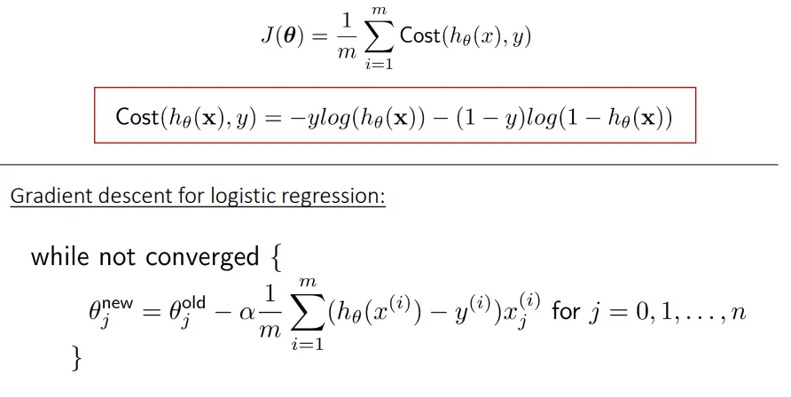
看起来你的一些东西混在了这里。在这样做时，关键是要跟踪向量的形状并确保你得到合理的结果。例如，你正在使用以下方法计算成本：

cost = ((-y) * np.log(sigmoid(X[i]))) - ((1 - y) * np.log(1 - sigmoid(X[i])))

在你的情况下，y 是一个有 20 项的向量，而 X[i] 是一个单一的值。这会使得你的成本计算成为一个 20 项的向量，这是没有意义的。你的成本应该是一个单一的值。（此外，在梯度下降函数中你还不必要地多次计算了这个成本）。

另外，如果你想让它适应你的数据，你需要给 X 添加偏置项。所以我们从那里开始吧。

X = np.asarray([
    [0.50],[0.75],[1.00],[1.25],[1.50],[1.75],[1.75],
    [2.00],[2.25],[2.50],[2.75],[3.00],[3.25],[3.50],
    [4.00],[4.25],[4.50],[4.75],[5.00],[5.50]])

ones = np.ones(X.shape)
X = np.hstack([ones, X])
# X.shape is now (20, 2)

现在Theta每个X需要2个值，因此初始化X和Y：

Y = np.array([0,0,0,0,0,0,1,0,1,0,1,0,1,0,1,1,1,1,1,1]).reshape([-1, 1])
# reshape Y so it's column vector so matrix multiplication is easier
Theta = np.array([[0], [0]])

你的Sigmoid函数很好。我们也可以制作一个向量化的成本函数：

def sigmoid(a):
    return 1.0 / (1 + np.exp(-a))

def cost(x, y, theta):
    m = x.shape[0]
    h = sigmoid(np.matmul(x, theta))
    cost = (np.matmul(-y.T, np.log(h)) - np.matmul((1 -y.T), np.log(1 - h)))/m
    return cost

成本函数有效的原因是因为Theta的形状为(2,1)，而X的形状为(20,2)，因此matmul(X, Theta)将被调整为(20,1)。然后将其与Y的转置矩阵相乘(y.T的形状为(1,20))，得到单个值，即给定特定Theta值时的成本。

然后我们可以编写一个函数来执行批量梯度下降的单个步骤：

def gradient_Descent(theta, alpha, x , y):
    m = x.shape[0]
    h = sigmoid(np.matmul(x, theta))
    grad = np.matmul(X.T, (h - y)) / m;
    theta = theta - alpha * grad
    return theta

注意：np.matmul(X.T, (h - y))正在计算形状为（2，20）和（20，1）的矩阵乘积，其结果为形状（2，1），这与Theta的形状相同，这就是您从梯度中想要的。这使您可以将其乘以学习速率并从初始的Theta中减去它，这就是梯度下降应该做的。

因此，现在您只需编写一个循环进行多次迭代，并更新Theta直到看起来收敛：

n_iterations = 500
learning_rate = 0.5

for i in range(n_iterations):
    Theta = gradient_Descent(Theta, learning_rate, X, Y)
    if i % 50 == 0:
        print(cost(X, Y, Theta))

这将在每50次迭代中打印成本，导致成本稳步下降，这正是您所希望的:

[[ 0.6410409]]
[[ 0.44766253]]
[[ 0.41593581]]
[[ 0.40697167]]
[[ 0.40377785]]
[[ 0.4024982]]
[[ 0.40195]]
[[ 0.40170533]]
[[ 0.40159325]]
[[ 0.40154101]]

你可以尝试不同的Theta初始值，你会发现它始终收敛到相同的结果。

现在你可以使用新找到的Theta值进行预测:

h = sigmoid(np.matmul(X, Theta))
print((h > .5).astype(int) )

这将输出与您的数据线性拟合的预期结果：

[[0]
 [0]
 [0]
 [0]
 [0]
 [0]
 [0]
 [0]
 [0]
 [0]
 [1]
 [1]
 [1]
 [1]
 [1]
 [1]
 [1]
 [1]
 [1]
 [1]]