如何拟合带有某些系数约束的多项式？

Question

使用NumPy的polyfit（或类似工具），有没有一种简单的方法可以获得一个解决方案，其中一个或多个系数被限制在特定值上？

例如，我们可以使用以下方式找到普通的多项式拟合：

x = np.array([0.0, 1.0, 2.0, 3.0,  4.0,  5.0])
y = np.array([0.0, 0.8, 0.9, 0.1, -0.8, -1.0])
z = np.polyfit(x, y, 3)

yielding

array([ 0.08703704, -0.81349206,  1.69312169, -0.03968254])

但是如果我想要最佳拟合多项式，其中第三个系数（在上面的例子中为z[2]）必须为1怎么办？我需要从头开始编写拟合吗？

- Jenny Shoars

---

我认为在这种情况下，您最好使用scipy的curve_fit函数或lmfit。 - Cleb

正如@Cleb所说，使用scipy.optimize.curve_fit()函数，并使用bounds参数来设置自变量的下限和上限。 - pault

Answer 1

在这种情况下，我会使用 curve_fit 或 lmfit；我将快速展示第一个选项。

import numpy as np
import matplotlib.pyplot as plt
from scipy.optimize import curve_fit

def func(x, a, b, c, d):
  return a + b * x + c * x ** 2 + d * x ** 3

x = np.array([0.0, 1.0, 2.0, 3.0,  4.0,  5.0])
y = np.array([0.0, 0.8, 0.9, 0.1, -0.8, -1.0])

print(np.polyfit(x, y, 3))

popt, _ = curve_fit(func, x, y)
print(popt)

popt_cons, _ = curve_fit(func, x, y, bounds=([-np.inf, 2, -np.inf, -np.inf], [np.inf, 2.001, np.inf, np.inf]))
print(popt_cons)

xnew = np.linspace(x[0], x[-1], 1000)

plt.plot(x, y, 'bo')
plt.plot(xnew, func(xnew, *popt), 'k-')
plt.plot(xnew, func(xnew, *popt_cons), 'r-')
plt.show()

这将打印出以下内容：

[ 0.08703704 -0.81349206  1.69312169 -0.03968254]
[-0.03968254  1.69312169 -0.81349206  0.08703704]
[-0.14331349  2.         -0.95913556  0.10494372]

在不受限制的情况下，polyfit和curve_fit给出相同的结果（只是顺序不同）。在受限制的情况下，所固定的参数为2，正如所期望的那样。图表如下：在lmfit中，您还可以选择某个参数是否应该被拟合，因此您也可以将其设置为所需值（请查看此答案）。

- Cleb

Answer 2

为了完整起见，使用 lmfit 的解决方案如下：

import numpy as np
import matplotlib.pyplot as plt
from lmfit import Model

def func(x, a, b, c, d):
    return a + b * x + c * x ** 2 + d * x ** 3

x = np.array([0.0, 1.0, 2.0, 3.0,  4.0,  5.0])
y = np.array([0.0, 0.8, 0.9, 0.1, -0.8, -1.0])

pmodel = Model(func)
params = pmodel.make_params(a=1, b=2, c=1, d=1)

params['b'].vary = False 

result = pmodel.fit(y, params, x=x)

print(result.fit_report())

xnew = np.linspace(x[0], x[-1], 1000)
ynew = result.eval(x=xnew)

plt.plot(x, y, 'bo')
plt.plot(x, result.best_fit, 'k-')
plt.plot(xnew, ynew, 'r-')
plt.show()

将打印一个全面的报告，包括不确定性、相关性和适合度统计数据，如下：

[[Model]]
    Model(func)
[[Fit Statistics]]
    # fitting method   = leastsq
    # function evals   = 10
    # data points      = 6
    # variables        = 3
    chi-square         = 0.066
    reduced chi-square = 0.022
    Akaike info crit   = -21.089
    Bayesian info crit = -21.714
[[Variables]]
    a:  -0.14331348 +/- 0.109441 (76.37%) (init= 1)
    b:   2 (fixed)
    c:  -0.95913555 +/- 0.041516 (4.33%) (init= 1)
    d:   0.10494371 +/- 0.008231 (7.84%) (init= 1)
[[Correlations]] (unreported correlations are <  0.100)
    C(c, d)                      = -0.987
    C(a, c)                      = -0.695
    C(a, d)                      =  0.610

并生成一个 的图形。

请注意，lmfit.Model相对于curve_fit有很多改进，包括根据函数参数自动命名参数，允许任何参数具有边界或仅被固定而不需要像上下边界几乎相等这样的无意义设置。关键在于lmfit使用具有属性的Parameter对象而不是普通的拟合变量数组。lmfit还支持数学约束、组合模型（例如添加或乘法模型）和优秀的报告。

- M Newville

---

这太棒了，特别是扩展统计信息和简洁的边界！我会收藏这篇文章以备将来参考。 - pault

Answer 3

很抱歉重新回答

但我觉得这个答案还有遗漏。

为了拟合多项式，我们需要解决以下方程组：

a0*x0^n + a1*x0^(n-1) .. + an*x0^0 = y0
a0*x1^n + a1*x1^(n-1) .. + an*x1^0 = y1
                 ...
a0*xm^n + a1*xm^(n-1) .. + an*xm^0 = ym

这是一个形式为V @ a = y的问题。

其中，"V"是一个范德蒙矩阵：

[[x0^n  x0^(n-1)  1],
 [x1^n  x1^(n-1)  1],
        ...
 [xm^n  xm^(n-1)  1]]

"y"是一个列向量，保存着y值：

[[y0],
 [y1],
  ...
 [ym]]

而 "a" 是我们要解决的系数列向量:

[[a0],
 [a1],
  ...
 [an]]

可以使用线性最小二乘法解决这个问题，具体步骤如下：

import numpy as np

x = np.array([0.0, 1.0, 2.0, 3.0,  4.0,  5.0])
y = np.array([0.0, 0.8, 0.9, 0.1, -0.8, -1.0])

deg = 3
V = np.vander(x, deg + 1)
z, *_ = np.linalg.lstsq(V, y, rcond=None)

print(z)
# [ 0.08703704 -0.81349206  1.69312169 -0.03968254]

...产生与polyfit方法相同的解决方案：

z = np.polyfit(x, y, deg)

print(z)
# [ 0.08703704 -0.81349206  1.69312169 -0.03968254]

我们希望找到一个解决方案，其中a2 = 1

将a2 = 1代入答案开头的方程组中，然后将相应项从左侧移到右侧，我们得到：

a0*x0^n + a1*x0^(n-1) + 1*x0^(n-2) .. + an*x0^0 = y0
a0*x1^n + a1*x1^(n-1) + 1*x0^(n-2) .. + an*x1^0 = y1
                 ...
a0*xm^n + a1*xm^(n-1) + 1*x0^(n-2) .. + an*xm^0 = ym

=>

a0*x0^n + a1*x0^(n-1) .. + an*x0^0 = y0 - 1*x0^(n-2)
a0*x1^n + a1*x1^(n-1) .. + an*x1^0 = y1 - 1*x0^(n-2)
                 ...
a0*xm^n + a1*xm^(n-1) .. + an*xm^0 = ym - 1*x0^(n-2)

这相当于从范德蒙矩阵中删除第二列，然后将其从y向量中减去，如下所示：

y_ = y - V[:, 2]
V_ = np.delete(V, 2, axis=1)
z_, *_ = np.linalg.lstsq(V_, y_, rcond=None)
z_ = np.insert(z_, 2, 1)

print(z_)
# [ 0.04659264 -0.48453866  1.          0.19438046]

请注意，在解决线性最小二乘问题后，我在系数向量中插入了1，因为我们不再解决a2，因为我们将其设置为1并从问题中删除了它。

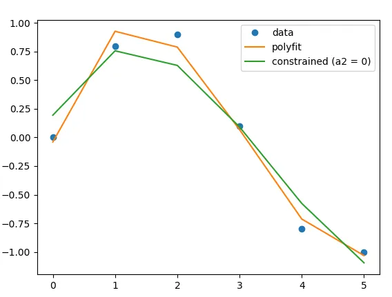
为了完整起见，这是绘制出来的解决方案：

以及我使用的完整代码：

import numpy as np

x = np.array([0.0, 1.0, 2.0, 3.0,  4.0,  5.0])
y = np.array([0.0, 0.8, 0.9, 0.1, -0.8, -1.0])

deg = 3
V = np.vander(x, deg + 1)
z, *_ = np.linalg.lstsq(V, y, rcond=None)

print(z)
# [ 0.08703704 -0.81349206  1.69312169 -0.03968254]

z = np.polyfit(x, y, deg)

print(z)
# [ 0.08703704 -0.81349206  1.69312169 -0.03968254]

y_ = y - V[:, 2]
V_ = np.delete(V, 2, axis=1)
z_, *_ = np.linalg.lstsq(V_, y_, rcond=None)
z_ = np.insert(z_, 2, 1)

print(z_)
# [ 0.04659264 -0.48453866  1.          0.19438046]

from matplotlib import pyplot as plt

plt.plot(x, y, 'o', label='data')
plt.plot(x, V @ z, label='polyfit')
plt.plot(x, V @ z_, label='constrained (a2 = 0)')

plt.legend()

plt.show()

- user9413641

Answer 4

以下是使用 scipy.optimize.curve_fit 实现的方法：

首先，让我们重新创建您的示例（作为一种合理性检查）：

import numpy as np
from scipy.optimize import curve_fit
​
def f(x, x3, x2, x1, x0):
    """this is the polynomial function"""
    return x0 + x1*x + x2*(x*x) + x3*(x*x*x)
​
popt, pcov = curve_fit(f, x, y)

print(popt)
#array([ 0.08703704, -0.81349206,  1.69312169, -0.03968254])

这与从np.polyfit()获得的值相匹配。

现在为x1添加约束条件：

popt, pcov = curve_fit(
    f, 
    x,
    y,
    bounds = ([-np.inf, -np.inf, .999999999, -np.inf], [np.inf, np.inf, 1.0, np.inf])
)
print(popt)
#array([ 0.04659264, -0.48453866,  1.        ,  0.19438046])

我必须使用.999999999，因为下限必须严格小于上限。

或者，您可以将带约束系数的函数定义为常量，并获取其他3个值：

def f_new(x, x3, x2, x0):
    x1 = 1
    return x0 + x1*x + x2*(x*x) + x3*(x*x*x)
popt, pcov = curve_fit(f_new, x, y)
print(popt)
#array([ 0.04659264, -0.48453866,  0.19438046])

- pault

Answer 5

这里有一种通用的方法，使用 scipy.optimize.curve_fit 来修复所需的多项式系数。

import numpy as np
from scipy.optimize import curve_fit

def polyfit(x, y, deg, which=-1, to=0):
    """
    An extension of ``np.polyfit`` to fix values of the vector 
    of polynomial coefficients. By default, the last coefficient 
    (i.e., the constant term) is kept at zero.

    Parameters
    ----------
    x : array_like
        x-coordinates of the sample points.
    y : array_like
        y-coordinates of the sample points.
    deg : int
        Degree of the fitting polynomial.
    which : int or array_like, optional
        Indexes of the coefficients to remain fixed. By default, -1.
    to : float or array_like, optional
        Values of the fixed coefficients. By default, 0.

    Returns
    -------
    np.ndarray
        (deg + 1) polynomial coefficients.
    """
    p0 = np.polyfit(x, y, deg)

    # if which == None it is reduced to np.polyfit
    if which is None: 
        return p0
    
    # indexes of the coeffs being fitted
    which_not = np.delete(np.arange(deg + 1), which)
    
    # create the array of coeffs
    def _fill_p(p):
        p_ = np.empty(deg + 1)  # empty array
        p_[which] = to          # fill with custom coeffs
        p_[which_not] = p       # fill with `p`
        return p_

    # callback function for fitting
    def _polyfit(x, *p):
        p_ = _fill_p(p)
        return np.polyval(p_, x)

    # get the array of coeffs
    p0 = np.delete(p0, which)                # use `p0` as initial condition
    p, _ = curve_fit(_polyfit, x, y, p0=p0)  # fitting
    p = _fill_p(p)                           # merge fixed and no-fixed coeffs
    return p

以下是如何使用上述函数的两个简单示例：

import matplotlib.pyplot as plt

# just create some fake data (a parabola)
np.random.seed(0)                               # seed to reproduce the example
deg = 2                                         # second order polynomial
p = np.random.randint(1, 5, size=deg+1)         # random vector of coefficients
x = np.linspace(0, 10, num=20)                  # fake data: x-array
y = np.polyval(p, x) + 1.5*np.random.randn(20)  # fake data: y-array
print(p)                                        # output:[1, 4, 2]

# fitting
p1 = polyfit(x, y, deg, which=2, to=p[2])        # case 1: last coeff is fixed
p2 = polyfit(x, y, deg, which=[1,2], to=p[1:3])  # case 2: last two coeffs are fixed
y1 = np.polyval(p1, x)                           # y-array for case 1
y2 = np.polyval(p2, x)                           # y-array for case 2
print(p1)                                        # output: [1.05, 3.67, 2.]
print(p2)                                        # output: [1.08, 4.,   2.]

# plotting
plt.plot(x, y, '.', label='fake data: y = p[0]*x**2 + p[1]*x + p[2]')
plt.plot(x, y1, label='p[2] fixed at 2')
plt.plot(x, y2, label='p[2] and p[1] fixed at [4, 2]')
plt.legend()
plt.show()

- alpelito7