假设我使用scipy/numpy创建了一个直方图,那么我就会有两个数组:一个用于存储每个区间内的计数,另一个用于存储区间边缘的值。如果我将这个直方图用作表示概率分布函数,如何从该分布中高效地生成随机数?
从直方图中生成随机数
39
- xvtk
2
你能澄清一下吗?你是想在每个直方图间隔内获得一定数量的随机数,还是想要基于直方图值的多项式插值的权重函数生成随机数? - Daniel
返回二进制中心就可以了,不需要插值或拟合。 - xvtk
7个回答
48
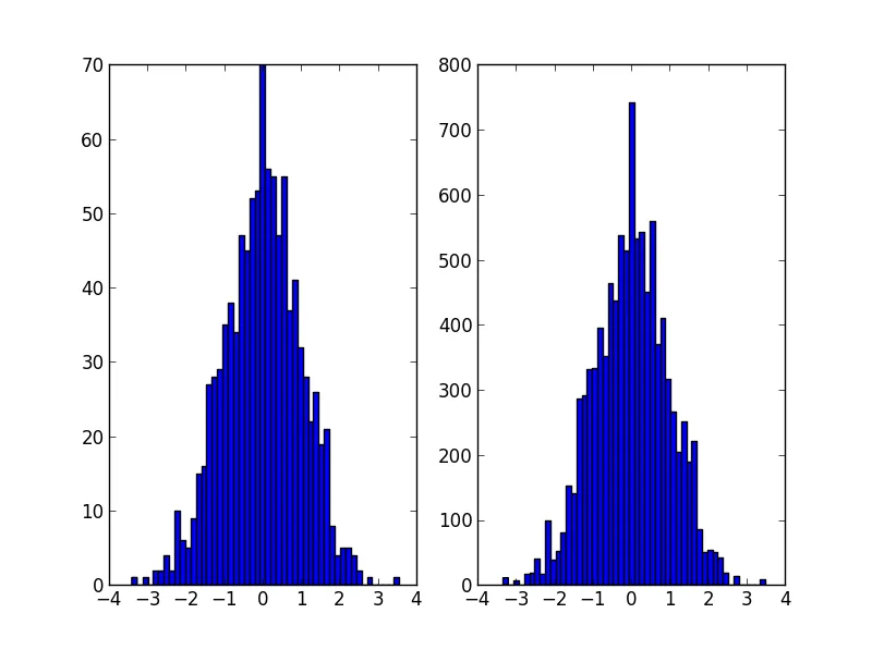
这可能就是 @Ophion 答案中的 np.random.choice 做的事情,但你可以构建一个标准化的累积密度函数,然后根据均匀随机数进行选择:
from __future__ import division
import numpy as np
import matplotlib.pyplot as plt

data = np.random.normal(size=1000)
hist, bins = np.histogram(data, bins=50)

bin_midpoints = bins[:-1] + np.diff(bins)/2
cdf = np.cumsum(hist)
cdf = cdf / cdf[-1]
values = np.random.rand(10000)
value_bins = np.searchsorted(cdf, values)
random_from_cdf = bin_midpoints[value_bins]

plt.subplot(121)
plt.hist(data, 50)
plt.subplot(122)
plt.hist(random_from_cdf, 50)
plt.show()
2D情况可按以下方式完成:
data = np.column_stack((np.random.normal(scale=10, size=1000),
                        np.random.normal(scale=20, size=1000)))
x, y = data.T
hist, x_bins, y_bins = np.histogram2d(x, y, bins=(50, 50))
x_bin_midpoints = x_bins[:-1] + np.diff(x_bins)/2
y_bin_midpoints = y_bins[:-1] + np.diff(y_bins)/2
cdf = np.cumsum(hist.ravel())
cdf = cdf / cdf[-1]

values = np.random.rand(10000)
value_bins = np.searchsorted(cdf, values)
x_idx, y_idx = np.unravel_index(value_bins,
                                (len(x_bin_midpoints),
                                 len(y_bin_midpoints)))
random_from_cdf = np.column_stack((x_bin_midpoints[x_idx],
                                   y_bin_midpoints[y_idx]))
new_x, new_y = random_from_cdf.T

plt.subplot(121, aspect='equal')
plt.hist2d(x, y, bins=(50, 50))
plt.subplot(122, aspect='equal')
plt.hist2d(new_x, new_y, bins=(50, 50))
plt.show()
- Jaime
5
是的,这肯定会起作用!它能推广到更高维度的直方图吗? - xvtk
1@xvtk 我已经用一个二维直方图编辑了我的答案。您应该能够将相同的方案应用于更高维度的分布。 - Jaime
1如果您正在使用Python 2,则需要添加“from future import division”导入,或将cdf归一化行更改为
cdf = cdf / float(cdf[-1])。 - Noam Peled
1你是完全正确的,Noam。这已经变得如此自然以至于我每次写Python代码时都把它作为第一行,以至于我总是忘记它不是标准行为。我已经编辑了我的答案。 - Jaime
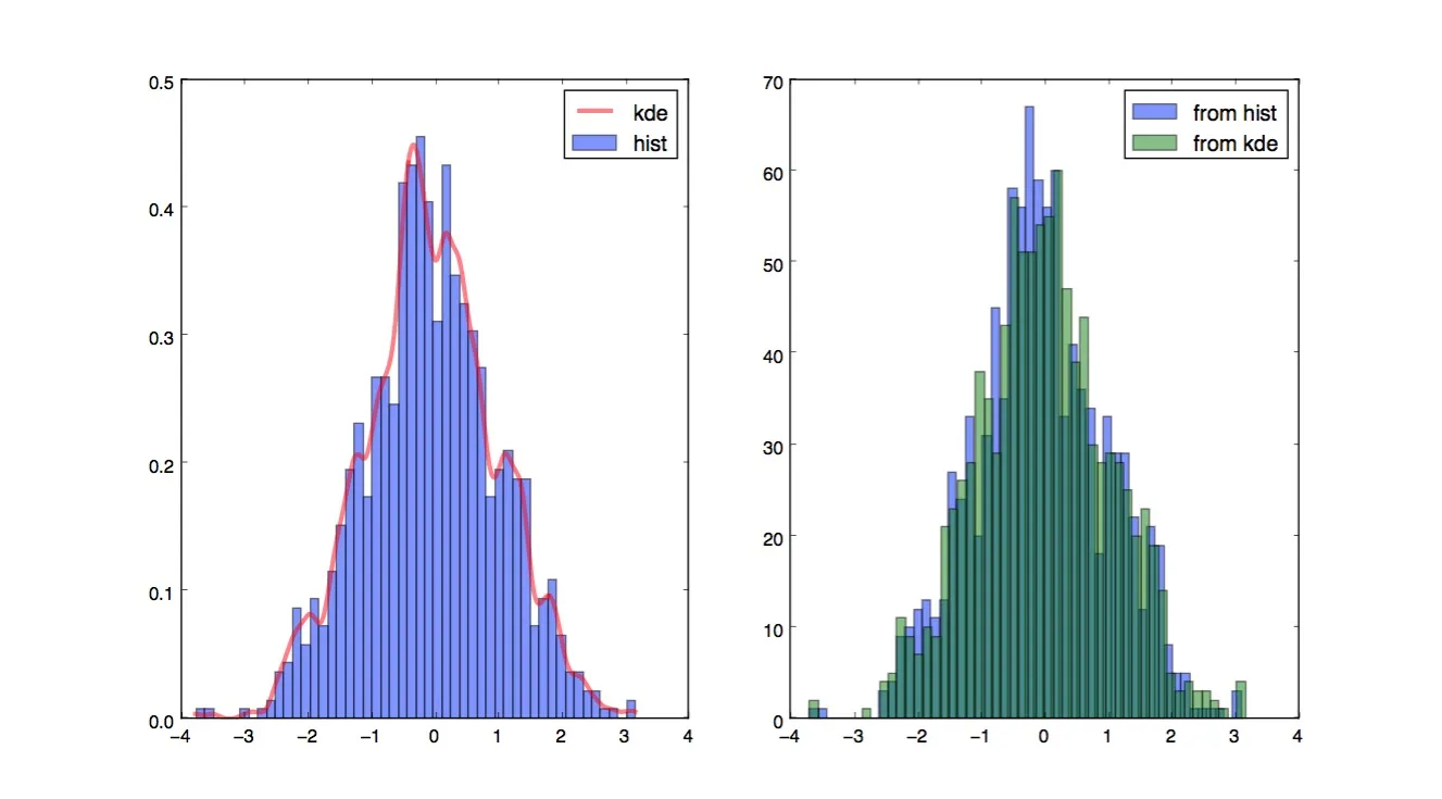
1我还在你的代码中添加了一个例子(作为新答案),演示如何从直方图的kde(核密度估计)生成随机数,这样可以更好地捕捉直方图的“生成器机制”。 - Noam Peled
27
@Jaime 的解决方案很棒,但你应该考虑使用直方图的核密度估计(kde)。在这里可以找到一个很好的解释,为什么在直方图上进行统计分析存在问题,以及为什么应该使用kde:这里
我编辑了@Jaime的代码,展示了如何使用来自scipy的kde。它看起来几乎一样,但更好地捕捉了直方图生成器。
from __future__ import division
import numpy as np
import matplotlib.pyplot as plt
from scipy.stats import gaussian_kde

def run():
    data = np.random.normal(size=1000)
    hist, bins = np.histogram(data, bins=50)

    x_grid = np.linspace(min(data), max(data), 1000)
    kdepdf = kde(data, x_grid, bandwidth=0.1)
    random_from_kde = generate_rand_from_pdf(kdepdf, x_grid)

    bin_midpoints = bins[:-1] + np.diff(bins) / 2
    random_from_cdf = generate_rand_from_pdf(hist, bin_midpoints)

    plt.subplot(121)
    plt.hist(data, 50, normed=True, alpha=0.5, label='hist')
    plt.plot(x_grid, kdepdf, color='r', alpha=0.5, lw=3, label='kde')
    plt.legend()
    plt.subplot(122)
    plt.hist(random_from_cdf, 50, alpha=0.5, label='from hist')
    plt.hist(random_from_kde, 50, alpha=0.5, label='from kde')
    plt.legend()
    plt.show()


def kde(x, x_grid, bandwidth=0.2, **kwargs):
    """Kernel Density Estimation with Scipy"""
    kde = gaussian_kde(x, bw_method=bandwidth / x.std(ddof=1), **kwargs)
    return kde.evaluate(x_grid)


def generate_rand_from_pdf(pdf, x_grid):
    cdf = np.cumsum(pdf)
    cdf = cdf / cdf[-1]
    values = np.random.rand(1000)
    value_bins = np.searchsorted(cdf, values)
    random_from_cdf = x_grid[value_bins]
    return random_from_cdf
- Noam Peled
1
你为什么要这样做
bw_method=bandwidth / x.std(ddof=1)?我认为应该是 bw_method=bandwidth * x.std(ddof=1),不是吗? - Fra11
也许就像这样。使用直方图的计数作为权重,并根据该权重选择索引值。
import numpy as np

initial=np.random.rand(1000)
values,indices=np.histogram(initial,bins=20)
values=values.astype(np.float32)
weights=values/np.sum(values)

#Below, 5 is the dimension of the returned array.
new_random=np.random.choice(indices[1:],5,p=weights)
print new_random

#[ 0.55141614  0.30226256  0.25243184  0.90023117  0.55141614]
- Daniel
4
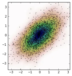
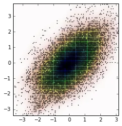
我有和OP相同的问题,我想分享我的解决方法。参考Jaime answer 和 Noam Peled answer,我使用核密度估计(KDE)解决了一个二维问题。
首先,让我们生成一些随机数据,然后从KDE中计算其概率密度函数(PDF)。我将使用SciPy中提供的示例来实现。
我们可以从这些新数据中计算出KDE并绘制它。
首先,让我们生成一些随机数据,然后从KDE中计算其概率密度函数(PDF)。我将使用SciPy中提供的示例来实现。
import numpy as np
import matplotlib.pyplot as plt
from scipy import stats

def measure(n):
    "Measurement model, return two coupled measurements."
    m1 = np.random.normal(size=n)
    m2 = np.random.normal(scale=0.5, size=n)
    return m1+m2, m1-m2

m1, m2 = measure(2000)
xmin = m1.min()
xmax = m1.max()
ymin = m2.min()
ymax = m2.max()

X, Y = np.mgrid[xmin:xmax:100j, ymin:ymax:100j]
positions = np.vstack([X.ravel(), Y.ravel()])
values = np.vstack([m1, m2])
kernel = stats.gaussian_kde(values)
Z = np.reshape(kernel(positions).T, X.shape)

fig, ax = plt.subplots()
ax.imshow(np.rot90(Z), cmap=plt.cm.gist_earth_r,
          extent=[xmin, xmax, ymin, ymax])
ax.plot(m1, m2, 'k.', markersize=2)
ax.set_xlim([xmin, xmax])
ax.set_ylim([ymin, ymax])
而情节是:
Z。# Generate the bins for each axis
x_bins = np.linspace(xmin, xmax, Z.shape[0]+1)
y_bins = np.linspace(ymin, ymax, Z.shape[1]+1)
# Find the middle point for each bin
x_bin_midpoints = x_bins[:-1] + np.diff(x_bins)/2
y_bin_midpoints = y_bins[:-1] + np.diff(y_bins)/2
# Calculate the Cumulative Distribution Function(CDF)from the PDF
cdf = np.cumsum(Z.ravel())
cdf = cdf / cdf[-1] # Normalização
# Create random data
values = np.random.rand(10000)
# Find the data position
value_bins = np.searchsorted(cdf, values)
x_idx, y_idx = np.unravel_index(value_bins,
(len(x_bin_midpoints),
len(y_bin_midpoints)))
# Create the new data
new_data = np.column_stack((x_bin_midpoints[x_idx],
y_bin_midpoints[y_idx]))
new_x, new_y = new_data.T
我们可以从这些新数据中计算出KDE并绘制它。
kernel = stats.gaussian_kde(new_data.T)
new_Z = np.reshape(kernel(positions).T, X.shape)

fig, ax = plt.subplots()
ax.imshow(np.rot90(new_Z), cmap=plt.cm.gist_earth_r,
          extent=[xmin, xmax, ymin, ymax])
ax.plot(new_x, new_y, 'k.', markersize=2)
ax.set_xlim([xmin, xmax])
ax.set_ylim([ymin, ymax])
- gabra
2
这里有一个解决方案,它返回在每个箱子内均匀分布的数据点而不是箱子中心点: "最初的回答"
def draw_from_hist(hist, bins, nsamples = 100000):
    cumsum = [0] + list(I.np.cumsum(hist))
    rand = I.np.random.rand(nsamples)*max(cumsum)
    return [I.np.interp(x, cumsum, bins) for x in rand]
- Arco Bast
0
对于@daniel, @arco-bast等人提出的解决方案,有些事情并不顺利。
以最后一个例子为例。
def draw_from_hist(hist, bins, nsamples = 100000):
    cumsum = [0] + list(I.np.cumsum(hist))
    rand = I.np.random.rand(nsamples)*max(cumsum)
    return [I.np.interp(x, cumsum, bins) for x in rand]
这假设至少第一个箱子没有内容,这可能是真的也可能不是。其次,这假设PDF的值位于箱子的上限,但实际上它大部分位于箱子的中心。
下面是另一种分为两部分的解决方案。
def init_cdf(hist,bins):
    """Initialize CDF from histogram

    Parameters
    ----------
        hist : array-like, float of size N
            Histogram height
        bins : array-like, float of size N+1
            Histogram bin boundaries

    Returns:
    --------
        cdf : array-like, float of size N+1
    """
    from numpy import concatenate, diff,cumsum

    # Calculate half bin sizes
    steps  = diff(bins) / 2  # Half bin size

    # Calculate slope between bin centres
    slopes = diff(hist) / (steps[:-1]+steps[1:])

    # Find height of end points by linear interpolation
    # - First part is linear interpolation from second over first
    #   point to lowest bin edge
    # - Second part is linear interpolation left neighbor to
    #   right neighbor up to but not including last point
    # - Third part is linear interpolation from second to last point
    #   over last point to highest bin edge
    # Can probably be done more elegant
    ends = concatenate(([hist[0] - steps[0] * slopes[0]],
                        hist[:-1] + steps[:-1] * slopes,
                        [hist[-1] + steps[-1] * slopes[-1]]))

    # Calculate cumulative sum
    sum = cumsum(ends)
    # Subtract off lower bound and scale by upper bound
    sum -= sum[0]
    sum /= sum[-1]

    # Return the CDF
    return sum

def sample_cdf(cdf,bins,size):
    """Sample a CDF defined at specific points.

    Linear interpolation between defined points

    Parameters
    ----------
       cdf : array-like, float, size N
           CDF evaluated at all points of bins. First and
           last point of bins are assumed to define the domain
           over which the CDF is normalized.
       bins : array-like, float, size N
           Points where the CDF is evaluated.  First and last points
           are assumed to define the end-points of the CDF's domain
       size : integer, non-zero
           Number of samples to draw
    Returns
    -------
        sample : array-like, float, of size ``size``
             Random sample
    """
    from numpy import interp
    from numpy.random import random

    return interp(random(size), cdf, bins)

# Begin example code
import numpy as np
import matplotlib.pyplot as plt

# initial histogram, coarse binning
hist,bins = np.histogram(np.random.normal(size=1000),np.linspace(-2,2,21))

# Calculate CDF, make sample, and new histogram w/finer binning
cdf = init_cdf(hist,bins)
sample = sample_cdf(cdf,bins,1000)
hist2,bins2 = np.histogram(sample,np.linspace(-3,3,61))

# Calculate bin centres and widths
mx = (bins[1:]+bins[:-1])/2
dx = np.diff(bins)
mx2 = (bins2[1:]+bins2[:-1])/2
dx2 = np.diff(bins2)

# Plot, taking care to show uncertainties and so on
plt.errorbar(mx,hist/dx,np.sqrt(hist)/dx,dx/2,'.',label='original')
plt.errorbar(mx2,hist2/dx2,np.sqrt(hist2)/dx2,dx2/2,'.',label='new')
plt.legend()
对不起,我不知道如何在StackOverflow上显示它,因此请复制并运行以查看要点。
- cholm
1
我的解决方案不假设第一个箱子为空。尝试使用
draw_from_hist([1],[0,1])。这将从区间[0,1]中均匀地绘制,如预期所示。 - Arco Bast0
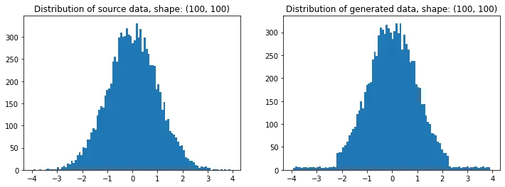
我在寻找一种基于另一个数组的分布生成随机数组的方法时,偶然发现了这个问题。如果使用numpy,我会调用random_like()函数。
然后我意识到,我已经编写了一个包Redistributor,它可能会为我完成这个任务,尽管该包的创建动机略有不同(Sklearn转换器能够将数据从任意分布转换为机器学习目的下的任意已知分布)。当然,我明白不需要必要的依赖关系,但至少知道这个包可能在将来对你有用。OP所问的事情在这里基本上是在幕后完成的。
警告:在幕后,所有操作都是在1D中完成的。该包还实现了多维包装器,但我没有使用它来编写此示例,因为我认为它太小众了。
安装:
pip install git+https://gitlab.com/paloha/redistributor
实现:
import numpy as np
import matplotlib.pyplot as plt

def random_like(source, bins=0, seed=None):
    from redistributor import Redistributor
    np.random.seed(seed)
    noise = np.random.uniform(source.min(), source.max(), size=source.shape)
    s = Redistributor(bins=bins, bbox=[source.min(), source.max()]).fit(source.ravel())
    s.cdf, s.ppf = s.source_cdf, s.source_ppf
    r = Redistributor(target=s, bbox=[noise.min(), noise.max()]).fit(noise.ravel())
    return r.transform(noise.ravel()).reshape(noise.shape)

source = np.random.normal(loc=0, scale=1, size=(100,100))
t = random_like(source, bins=80) # More bins more precision (0 = automatic)

# Plotting
plt.figure(figsize=(12,4))
plt.subplot(121); plt.title(f'Distribution of source data, shape: {source.shape}')
plt.hist(source.ravel(), bins=100)
plt.subplot(122); plt.title(f'Distribution of generated data, shape: {t.shape}')
plt.hist(t.ravel(), bins=100); plt.show()
解释:
import numpy as np
import matplotlib.pyplot as plt
from redistributor import Redistributor
from sklearn.metrics import mean_squared_error

# We have some source array with "some unknown" distribution (e.g. an image)
# For the sake of example we just generate a random gaussian matrix
source = np.random.normal(loc=0, scale=1, size=(100,100))
plt.figure(figsize=(12,4))
plt.subplot(121); plt.title('Source data'); plt.imshow(source, origin='lower')
plt.subplot(122); plt.title('Source data hist'); plt.hist(source.ravel(), bins=100); plt.show()

# We want to generate a random matrix from the distribution of the source
# So we create a random uniformly distributed array called noise
noise = np.random.uniform(source.min(), source.max(), size=(100,100))
plt.figure(figsize=(12,4))
plt.subplot(121); plt.title('Uniform noise'); plt.imshow(noise, origin='lower')
plt.subplot(122); plt.title('Uniform noise hist'); plt.hist(noise.ravel(), bins=100); plt.show()

# Then we fit (approximate) the source distribution using Redistributor
# This step internally approximates the cdf and ppf functions.
s = Redistributor(bins=200, bbox=[source.min(), source.max()]).fit(source.ravel())

# A little naming workaround to make obj s work as a target distribution
s.cdf = s.source_cdf
s.ppf = s.source_ppf

# Here we create another Redistributor but now we use the fitted Redistributor s as a target
r = Redistributor(target=s, bbox=[noise.min(), noise.max()])

# Here we fit the Redistributor r to the noise array's distribution
r.fit(noise.ravel())

# And finally, we transform the noise into the source's distribution
t = r.transform(noise.ravel()).reshape(noise.shape)
plt.figure(figsize=(12,4))
plt.subplot(121); plt.title('Transformed noise'); plt.imshow(t, origin='lower')
plt.subplot(122); plt.title('Transformed noise hist'); plt.hist(t.ravel(), bins=100); plt.show()

# Computing the difference between the two arrays
print('Mean Squared Error between source and transformed: ', mean_squared_error(source, t))
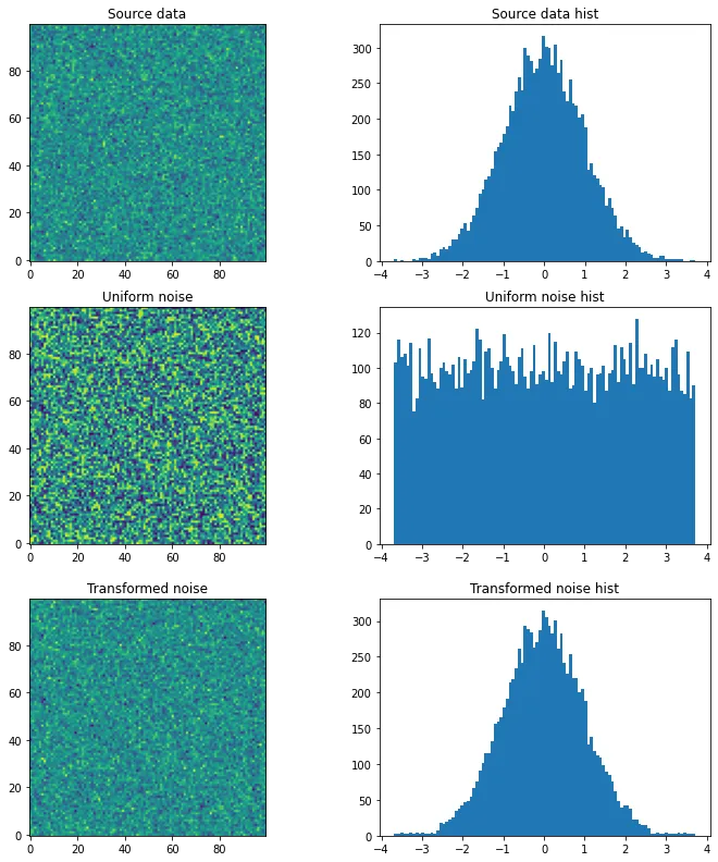
源数据和转换后的均方误差为:2.0574123162302143
- Paloha
网页内容由stack overflow 提供, 点击上面的可以查看英文原文,
原文链接
原文链接