为什么手动计算的ggplot2 95％CI和预测95％CI不同？

Question

我想知道为什么在从线性混合效应模型计算95%置信带时，ggplot2生成的带比手动计算的带更窄，例如按照Ben Bolker在这里的方法进行计算predictions的置信区间。也就是说，ggplot2是否给出了模型的不准确表示？

下面是使用sleepstudy数据集的可重现示例（已修改为与我正在处理的df结构相似）：

data("sleepstudy") # load dataset 
height <- seq(165, 185, length.out = 18) # create vector called height
Treatment <- rep(c("Control", "Drug"), 9) # create vector called treatment
Subject <- levels(sleepstudy$Subject) # get vector of Subject
ht.subject <- data.frame(height, Subject, Treatment) 
sleepstudy <- dplyr::left_join(sleepstudy, ht.subject, by="Subject") # Append df so that each subject has its own height and treatment
sleepstudy$Treatment <- as.factor(sleepstudy$Treatment)

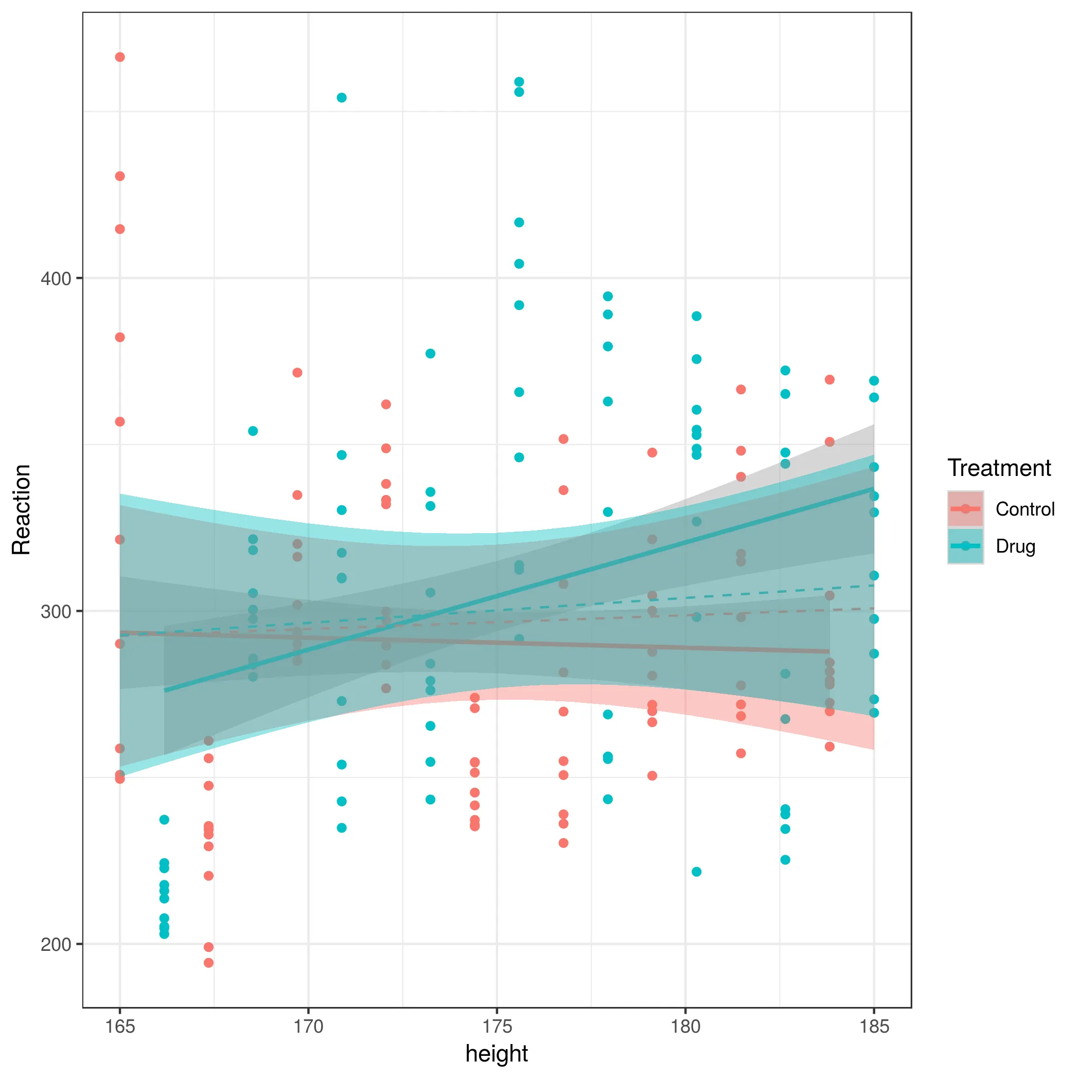
生成模型，将预测结果添加到原始数据框中，并绘制图表。

m.sleep <- lmer(Reaction ~ Treatment*height + (1 + Days|Subject), data=sleepstudy)
sleepstudy$pred <- predict(m.sleep)
ggplot(sleepstudy, aes(height, pred, col=Treatment)) + geom_smooth(method="lm")[2] 

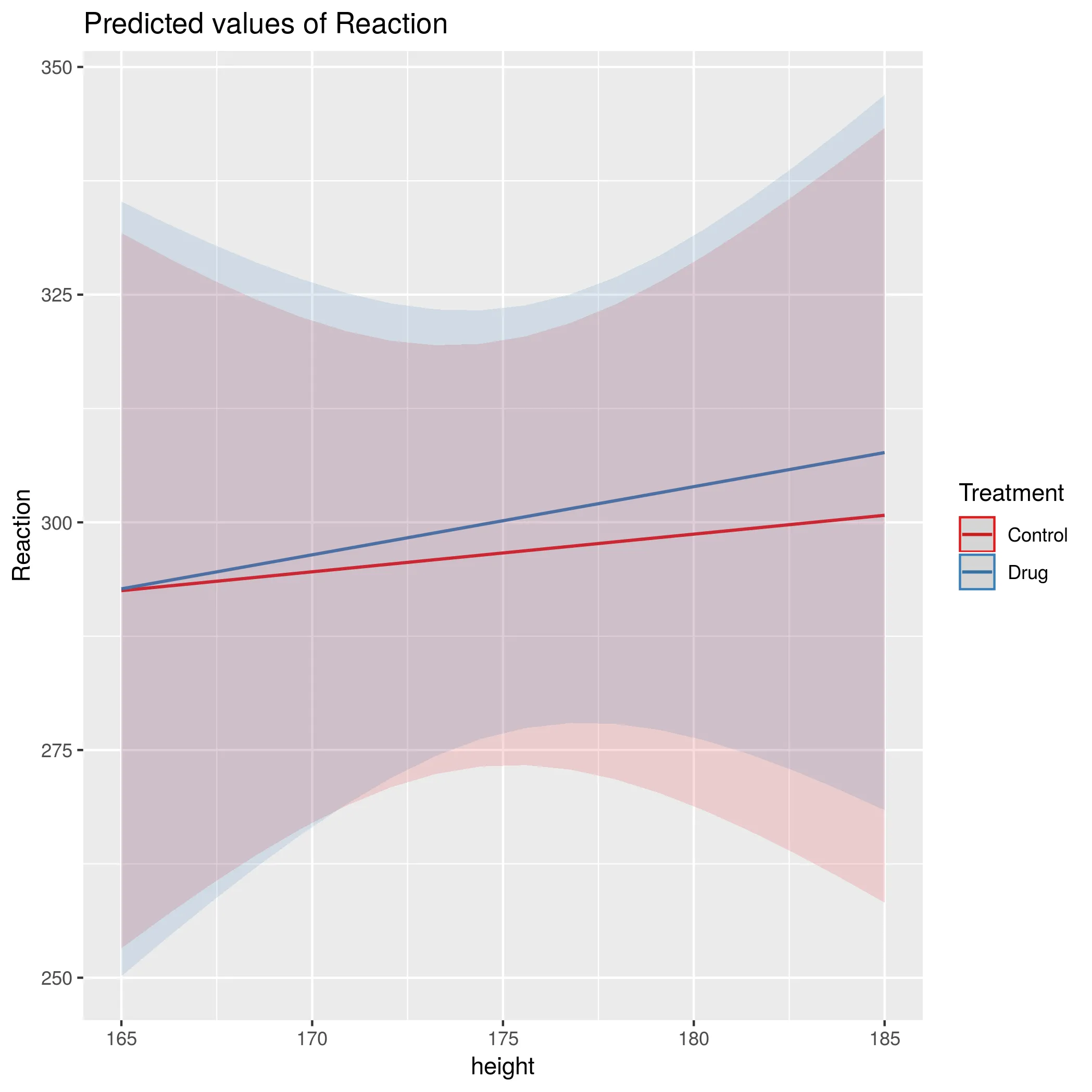
使用Bolker方法计算置信区间

newdf <- expand.grid(height=seq(165, 185, 1),
                   Treatment=c("Control","Drug"))
newdf$Reaction <- predict(m.sleep, newdf, re.form=NA) 
modmat <- model.matrix(terms(m.sleep), newdf)
pvar1 <- diag(modmat %*% tcrossprod(vcov(m.sleep), modmat))
tvar1 <- pvar1+VarCorr(m.sleep)$Subject[1]
cmult <- 1.96

newdf <- data.frame(newdf
,plo = newdf$Reaction-cmult*sqrt(pvar1)
,phi = newdf$Reaction+cmult*sqrt(pvar1)
,tlo = newdf$Reaction-cmult*sqrt(tvar1)
,thi = newdf$Reaction+cmult*sqrt(tvar1))

# plot confidence intervals
ggplot(newdf, aes(x=height, y=Reaction, colour=Treatment)) + 
geom_point() +
geom_ribbon(aes(ymin=plo, ymax=phi, fill=Treatment), alpha=0.4)[2]

- S.Bird

---

这可能是一个适合在stats.stackexchange.com上提问的问题。快速浏览了一下你的代码和链接的GitHub页面之后，我的疑问是：Bolker的方法是否生成关于预测值的_置信_区间还是_预测_区间？大多数统计软件会区分这两者。 - Kevin Troy

我认为这是用于生成关于预测的置信区间，但也许我对此有所误解。我会按照你的建议重新发布在stats.stackexchange上。 - S.Bird

Answer 1

通过一些微调，这似乎是一致的。置信区间确实更大，但并没有非常大。请记住，ggplot正在拟合一个非常不同的模型；它正在拟合分别针对治疗的线性模型（而不是线性混合模型），这些模型忽略了（1）重复测量和（2）天数的影响。

拟合具有随机斜率但无总体斜率的模型似乎很奇怪（例如，见此处），因此我添加了一个固定效应Days：

m.sleep <- lmer(Reaction ~ Treatment*height + Days +
                (1 + Days|Subject),
                data=sleepstudy)

我稍微重新组织了绘图代码：

theme_set(theme_bw())
gg0 <- ggplot(sleepstudy, aes(height, colour=Treatment)) +
    geom_point(aes(y=Reaction))+
    geom_smooth(aes(y=pred), method="lm")

• 如果您想计算置信区间（这与lm()/ggplot2正在做的相比较），那么您可能不应该在方差中添加 VarCorr(m.sleep)$Subject[1] （ FAQ示例 中的 tvar1 变量是用于创建预测区间而不是置信区间...）
• 由于上面的模型中有 Days，所以我将 mean(sleepstudy$Days) 添加到预测数据框中。

newdf <- expand.grid(height=seq(165, 185, 1),
                     Treatment=c("Control","Drug"),
                     Days=mean(sleepstudy$Days))
newdf$Reaction <- newdf$pred <- predict(m.sleep, newdf, re.form=NA) 
modmat <- model.matrix(terms(m.sleep), newdf)
pvar1 <- diag(modmat %*% tcrossprod(vcov(m.sleep), modmat))
tvar1 <- pvar1
cmult <- 1.96

newdf <- data.frame(newdf
,plo = newdf$Reaction-cmult*sqrt(pvar1)
,phi = newdf$Reaction+cmult*sqrt(pvar1)
,tlo = newdf$Reaction-cmult*sqrt(tvar1)
,thi = newdf$Reaction+cmult*sqrt(tvar1))

gg0 + 
    geom_point(data=newdf,aes(y=Reaction)) +
    geom_ribbon(data=newdf,
                aes(ymin=plo, ymax=phi, fill=Treatment), alpha=0.4,
                colour=NA)

与估计的斜率和标准误差相比较：

m0 <- lm(Reaction~height*Treatment,sleepstudy)
ff <- function(m) {
    print(coef(summary(m))[-1,c("Estimate","Std. Error")],digits=2)
}

> ff(m0)
##                      Estimate Std. Error
## height                   -0.3       0.94
## TreatmentDrug          -602.2     234.01
## height:TreatmentDrug      3.5       1.34

ff(m.sleep)
##                      Estimate Std. Error
## TreatmentDrug          -55.03      425.3
## height                   0.41        1.7
## Days                    10.47        1.5
## TreatmentDrug:height     0.33        2.4

这看起来是一致的/正确的：混合模型在高度与斜率以及高度:治疗交互作用方面提供了更大的标准误差。(因为TreatmentDrug的主效应是在height==0处预期的治疗效应，所以它们看起来很疯狂...)

---

作为交叉验证，我可以使用sjPlot::plot_model()获得类似的答案...

library(sjPlot)
plot_model(m.sleep, type="pred", terms=c("height","Treatment"))

- Ben Bolker