亲爱的stackoverflow用户们,
我正在尝试计算由一组3D点定义的任意(但光滑)表面上的法向量。为此,我使用平面拟合算法,该算法基于我计算法向量的点的10个最近邻点找到局部最小二乘平面。
然而,它并不总是找到看起来最好的平面。因此,我想知道我的实现或算法是否存在缺陷。我使用奇异值分解,因为我在有关平面拟合的几个链接中发现了推荐。下面是一段可以在我的机器上重现这种行为的代码:
结果是: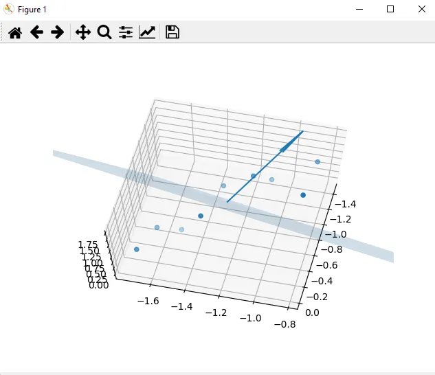 我希望它更像这样:
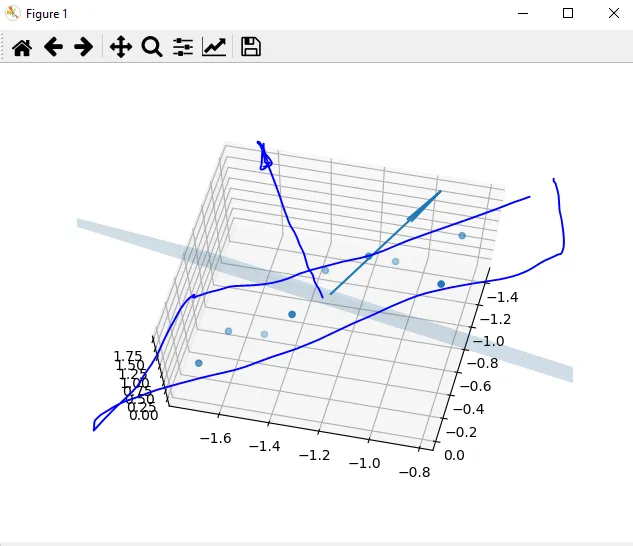 (对于不好的草图,我很抱歉)
那么,这里有什么问题呢?可能是我的matplotlib代码中的显示错误吗?
祝一切顺利!
我正在尝试计算由一组3D点定义的任意(但光滑)表面上的法向量。为此,我使用平面拟合算法,该算法基于我计算法向量的点的10个最近邻点找到局部最小二乘平面。
然而,它并不总是找到看起来最好的平面。因此,我想知道我的实现或算法是否存在缺陷。我使用奇异值分解,因为我在有关平面拟合的几个链接中发现了推荐。下面是一段可以在我的机器上重现这种行为的代码:
#library imports
import numpy as np
import math
import matplotlib.pyplot    as     plt
from   mpl_toolkits.mplot3d import Axes3D

#values used for best plane fit
xyz = np.array([[-1.04194694, -1.17965867,  1.09517722],
[-0.39947906, -1.37104542,  1.36019265],
[-1.0634807 , -1.35020616,  0.46773962],
[-0.48640524, -1.64476106,  0.2726187 ],
[-0.05720509, -1.6791781 ,  0.76964551],
[-1.27522669, -1.10240358,  0.33761405],
[-0.61274031, -1.52709874, -0.09945502],
[-1.402693  , -0.86807757,  0.88866091],
[-0.72520241, -0.86800727,  1.69729388]])

''' best plane fit'''
#1.calculate centroid of points and make points relative to it
centroid         = xyz.mean(axis = 0)
xyzT             = np.transpose(xyz)
xyzR             = xyz - centroid                         #points relative to centroid
xyzRT            = np.transpose(xyzR)

#2. calculate the singular value decomposition of the xyzT matrix and get the normal as the last column of u matrix
u, sigma, v       = np.linalg.svd(xyzRT)
normal            = u[2]
normal            = normal / np.linalg.norm(normal)       #we want normal vectors normalized to unity

'''matplotlib display'''
#prepare normal vector for display
forGraphs = list()
forGraphs.append(np.array([centroid[0],centroid[1],centroid[2],normal[0],normal[1], normal[2]]))

#get d coefficient to plane for display
d = normal[0] * centroid[0] + normal[1] * centroid[1] + normal[2] * centroid[2]

# create x,y for display
minPlane = int(math.floor(min(min(xyzT[0]), min(xyzT[1]), min(xyzT[2]))))
maxPlane = int(math.ceil(max(max(xyzT[0]), max(xyzT[1]), max(xyzT[2]))))
xx, yy = np.meshgrid(range(minPlane,maxPlane), range(minPlane,maxPlane))

# calculate corresponding z for display
z = (-normal[0] * xx - normal[1] * yy + d) * 1. /normal[2]

#matplotlib display code
forGraphs = np.asarray(forGraphs)
X, Y, Z, U, V, W = zip(*forGraphs)
fig = plt.figure()
ax = fig.add_subplot(111, projection='3d')
ax.plot_surface(xx, yy, z, alpha=0.2)
ax.scatter(xyzT[0],xyzT[1],xyzT[2])
ax.quiver(X, Y, Z, U, V, W)
ax.set_xlim([min(xyzT[0])- 0.1, max(xyzT[0]) + 0.1])
ax.set_ylim([min(xyzT[1])- 0.1, max(xyzT[1]) + 0.1])
ax.set_zlim([min(xyzT[2])- 0.1, max(xyzT[2]) + 0.1])
plt.show()
结果是:
我希望它更像这样:
(对于不好的草图,我很抱歉)那么,这里有什么问题呢?可能是我的matplotlib代码中的显示错误吗?
祝一切顺利!