如何从curve_fit获取置信区间

Question

我的问题涉及到统计学和Python，我在两个方面都是初学者。我正在运行一个模拟，对于每个自变量（X）的值，我会生成1000个因变量（Y）的值。我所做的是为每个X的值计算Y的平均值，并使用scipy.optimize.curve_fit拟合这些平均值。曲线拟合得很好，但我也想画出置信区间。我不确定我所做的是否正确或者我想做的是否可行，但我的问题是如何从curve_fit产生的协方差矩阵中获得置信区间。该代码首先从文件中读取平均值，然后简单地使用curve_fit。

import numpy as np
import matplotlib.pyplot as plt
from scipy.optimize import curve_fit


def readTDvsTx(L, B, P, fileformat):
    # L should be '_Fixed_' or '_'
    TD = []
    infile = open(fileformat.format(L, B, P), 'r')
    infile.readline()  # To remove header
    for line in infile:
        l = line.split()  # each line contains TxR followed by CD followed by TD
        if eval(l[0]) >= 70 and eval(l[0]) <=190:
            td = eval(l[2])
            TD.append(td)
    infile.close()
    tdArray = np.array(TD)

    return tdArray


def rec(x, a, b):
    return a * (1 / (x**2)) + b



fileformat = 'Densities_file{}BS{}_PRNTS{}.txt'
txR = np.array(range(70, 200, 20))
parents = np.array(range(1,6))
disc_p1 = readTDvsTx('_Fixed_', 5, 1, fileformat)


popt, pcov = curve_fit(rec, txR, disc_p1)


plt.plot(txR, rec(txR, popt[0], popt[1]), 'r-')
plt.plot(txR, disc_p1, '.')

print(popt)
plt.show()

这是拟合后的结果：

- osmak

---

kmpfit模块可以在拟合非线性函数时计算置信区间，详情请参阅我此回答。您需要使用所有点进行拟合，而不仅仅是平均值。 - Ulrich Stern

如果您想自己进行置信区间的计算，我的回答中有一个链接（指向此页面：http://www.graphpad.com/guides/prism/7/curve-fitting/index.htm?reg_how_confidence_and_prediction_.htm）。 - Ulrich Stern

使用所有点进行拟合并不是那么简单，因为osmak的函数是多元的。 - Vlas Sokolov

感谢大家的评论。问题是我认为我误解了获取值的方式。在我的模拟中，我搜索某个密度，我称之为目标密度或TD。我这样做的方式是运行1000个模拟实例，并使用某些标准检查这些实例的平均值，如果满足条件，则表示我已经达到了我的TD。增加自变量的值不会影响TD，即它不是正态分布的。 - osmak

Answer 1

以下是一个快速但错误的答案: 您可以将您的a和b参数的误差近似为其对角线的平方根： np.sqrt(np.diagonal(pcov))，并使用参数不确定性来绘制置信区间。

该答案是错误的，因为在拟合数据到模型之前，您需要对平均disc_p1点上的误差进行估计。当进行平均时，您已经丢失了关于总体散布的信息，导致curve_fit相信您提供的y点是绝对且无可争议的。这可能会导致您的参数误差被低估。

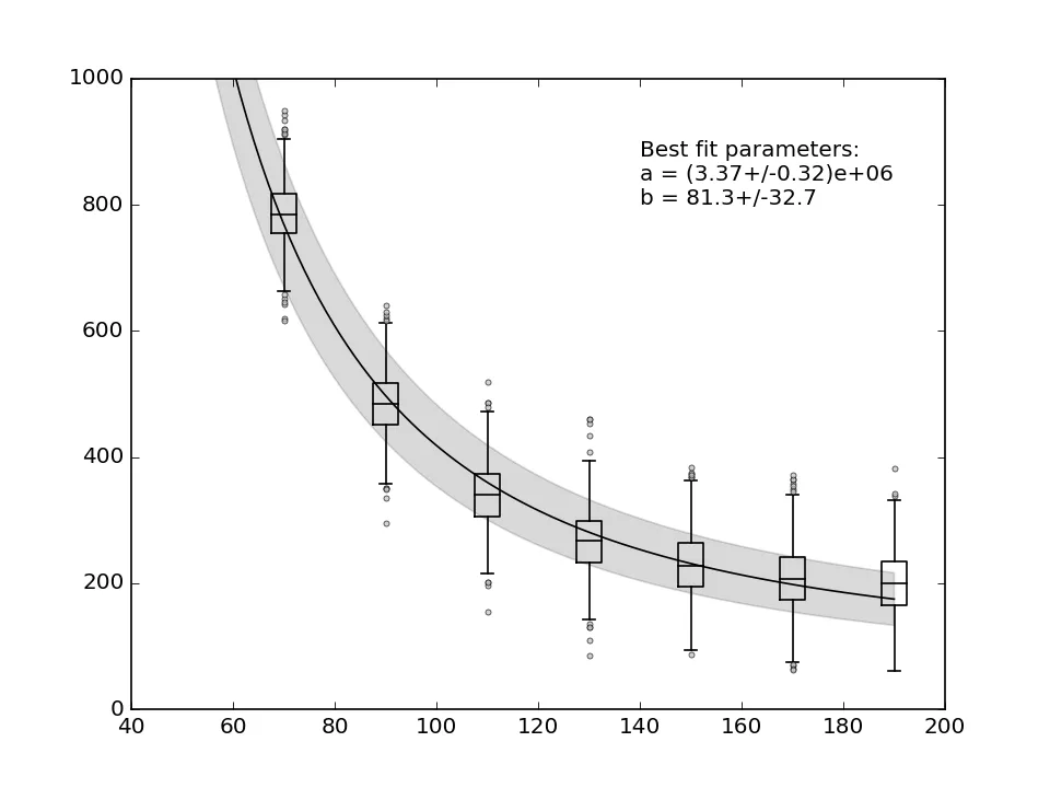
要估计平均Y值的不确定性，您需要估计它们的离散度量，并在向curve_fit传递它时表示您的误差是绝对的。下面是一个示例，展示了如何对一个随机数据集执行此操作，其中每个点由从正态分布中抽取的1000个样本组成。

from scipy.optimize import curve_fit
import matplotlib.pylab as plt
import numpy as np

# model function
func = lambda x, a, b: a * (1 / (x**2)) + b 

# approximating OP points
n_ypoints = 7 
x_data = np.linspace(70, 190, n_ypoints)

# approximating the original scatter in Y-data
n_nested_points = 1000
point_errors = 50
y_data = [func(x, 4e6, -100) + np.random.normal(x, point_errors,
          n_nested_points) for x in x_data]

# averages and dispersion of data
y_means = np.array(y_data).mean(axis = 1)
y_spread = np.array(y_data).std(axis = 1)

best_fit_ab, covar = curve_fit(func, x_data, y_means,
                               sigma = y_spread,
                               absolute_sigma = True)
sigma_ab = np.sqrt(np.diagonal(covar))

from uncertainties import ufloat
a = ufloat(best_fit_ab[0], sigma_ab[0])
b = ufloat(best_fit_ab[1], sigma_ab[1])
text_res = "Best fit parameters:\na = {}\nb = {}".format(a, b)
print(text_res)

# plotting the unaveraged data
flier_kwargs = dict(marker = 'o', markerfacecolor = 'silver',
                    markersize = 3, alpha=0.7)
line_kwargs = dict(color = 'k', linewidth = 1)
bp = plt.boxplot(y_data, positions = x_data,
                 capprops = line_kwargs,
                 boxprops = line_kwargs,
                 whiskerprops = line_kwargs,
                 medianprops = line_kwargs,
                 flierprops = flier_kwargs,
                 widths = 5,
                 manage_ticks = False)
# plotting the averaged data with calculated dispersion
#plt.scatter(x_data, y_means, facecolor = 'silver', alpha = 1)
#plt.errorbar(x_data, y_means, y_spread, fmt = 'none', ecolor = 'black')

# plotting the model
hires_x = np.linspace(50, 190, 100)
plt.plot(hires_x, func(hires_x, *best_fit_ab), 'black')
bound_upper = func(hires_x, *(best_fit_ab + sigma_ab))
bound_lower = func(hires_x, *(best_fit_ab - sigma_ab))
# plotting the confidence intervals
plt.fill_between(hires_x, bound_lower, bound_upper,
                 color = 'black', alpha = 0.15)
plt.text(140, 800, text_res)
plt.xlim(40, 200)
plt.ylim(0, 1000)
plt.show()

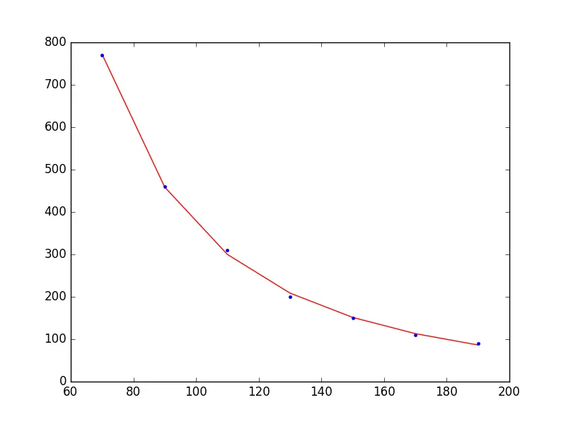
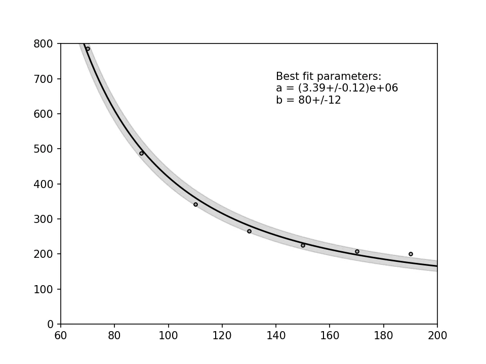
编辑： 如果您不考虑数据点上的内在误差，那么使用我之前提到的“快速而错误”的情况可能就足够了。然后可以使用协方差矩阵的对角线条目的平方根来计算置信区间。但是请注意，由于我们丢弃了不确定性，所以置信区间现在已经缩小了：

from scipy.optimize import curve_fit
import matplotlib.pylab as plt
import numpy as np

func = lambda x, a, b: a * (1 / (x**2)) + b

n_ypoints = 7
x_data = np.linspace(70, 190, n_ypoints)

y_data = np.array([786.31, 487.27, 341.78, 265.49,
                    224.76, 208.04, 200.22])
best_fit_ab, covar = curve_fit(func, x_data, y_data)
sigma_ab = np.sqrt(np.diagonal(covar))

# an easy way to properly format parameter errors
from uncertainties import ufloat
a = ufloat(best_fit_ab[0], sigma_ab[0])
b = ufloat(best_fit_ab[1], sigma_ab[1])
text_res = "Best fit parameters:\na = {}\nb = {}".format(a, b)
print(text_res)

plt.scatter(x_data, y_data, facecolor = 'silver',
            edgecolor = 'k', s = 10, alpha = 1)

# plotting the model
hires_x = np.linspace(50, 200, 100)
plt.plot(hires_x, func(hires_x, *best_fit_ab), 'black')
bound_upper = func(hires_x, *(best_fit_ab + sigma_ab))
bound_lower = func(hires_x, *(best_fit_ab - sigma_ab))
# plotting the confidence intervals
plt.fill_between(hires_x, bound_lower, bound_upper,
                 color = 'black', alpha = 0.15)
plt.text(140, 630, text_res)
plt.xlim(60, 200)
plt.ylim(0, 800)
plt.show()

如果您不确定是否应包括绝对误差或如何在您的情况下估计它们，最好在Cross Validated上寻求建议，因为Stack Overflow主要用于回归方法实现的讨论，而不是关于底层统计学的讨论。

- Vlas Sokolov

---

谢谢你的回答。问题是我认为我误解了获取值的方式。在我的模拟中，我搜索一定密度，我称之为目标密度或TD。我这样做的方式是运行1000个模拟实例，并使用某些标准检查这些实例的平均值，如果满足，则表示我已经达到了我的TD。增加自变量的值不会影响TD，即它不是正态分布的。 - osmak

那么收敛的 TD 值就没有任何不确定性了吗？ - Vlas Sokolov

@Steve，matplotlib的API发生了变化，在更新版本中，manage_xticks变成了manage_ticks。 - Vlas Sokolov

协方差矩阵的对角线元素的平方根可以用来计算置信区间，但这样做是否忽略了参数之间的协方差？我该如何考虑它们的影响？ - Joachim Breitner

@JoachimBreitner 是的，那基本上是一个隐含的假设，因为我使用了 np.diagonal。如果你的参数空间不平凡，你不应该使用像这样的点估计方法，而应该使用能够对整个参数空间进行采样的方法。贝叶斯方法通常很适用。但再次强调，我不是统计学家，所以不能确定 :) - Vlas Sokolov