我有许多元组(par1, par2),即从多次重复实验中获得的二维参数空间中的点。
我正在寻找一种计算和可视化置信椭圆的方法(不确定这是否是正确术语)。下面是我在网上找到的一个示例图来说明我的意思:
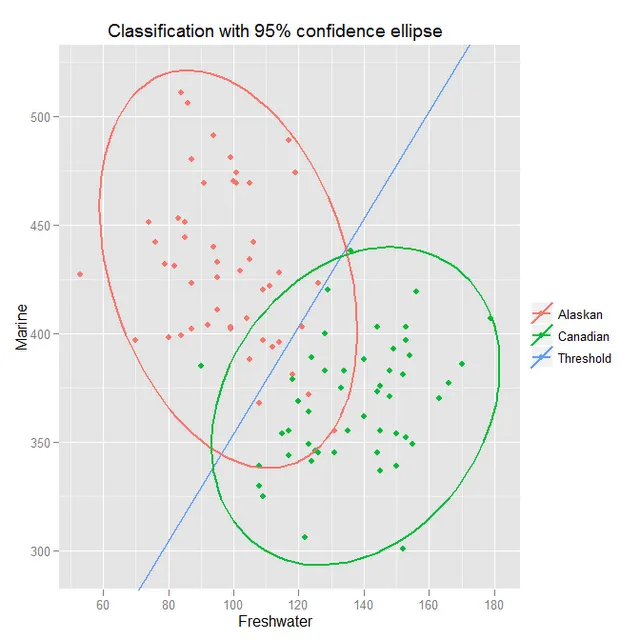
来源: blogspot.ch/2011/07/classification-and-discrimination-with.html
因此,原则上需要将多元正态分布拟合到数据点的二维直方图中。有人能帮我吗?
我有许多元组(par1, par2),即从多次重复实验中获得的二维参数空间中的点。
我正在寻找一种计算和可视化置信椭圆的方法(不确定这是否是正确术语)。下面是我在网上找到的一个示例图来说明我的意思:
来源: blogspot.ch/2011/07/classification-and-discrimination-with.html
因此,原则上需要将多元正态分布拟合到数据点的二维直方图中。有人能帮我吗?
听起来你只是想要散点图的2-sigma椭圆?
如果是的话,考虑像这样做(参考这里的一些论文代码:https://github.com/joferkington/oost_paper_code/blob/master/error_ellipse.py):
import numpy as np
import matplotlib.pyplot as plt
from matplotlib.patches import Ellipse
def plot_point_cov(points, nstd=2, ax=None, **kwargs):
"""
Plots an `nstd` sigma ellipse based on the mean and covariance of a point
"cloud" (points, an Nx2 array).
Parameters
----------
points : An Nx2 array of the data points.
nstd : The radius of the ellipse in numbers of standard deviations.
Defaults to 2 standard deviations.
ax : The axis that the ellipse will be plotted on. Defaults to the
current axis.
Additional keyword arguments are pass on to the ellipse patch.
Returns
-------
A matplotlib ellipse artist
"""
pos = points.mean(axis=0)
cov = np.cov(points, rowvar=False)
return plot_cov_ellipse(cov, pos, nstd, ax, **kwargs)
def plot_cov_ellipse(cov, pos, nstd=2, ax=None, **kwargs):
"""
Plots an `nstd` sigma error ellipse based on the specified covariance
matrix (`cov`). Additional keyword arguments are passed on to the
ellipse patch artist.
Parameters
----------
cov : The 2x2 covariance matrix to base the ellipse on
pos : The location of the center of the ellipse. Expects a 2-element
sequence of [x0, y0].
nstd : The radius of the ellipse in numbers of standard deviations.
Defaults to 2 standard deviations.
ax : The axis that the ellipse will be plotted on. Defaults to the
current axis.
Additional keyword arguments are pass on to the ellipse patch.
Returns
-------
A matplotlib ellipse artist
"""
def eigsorted(cov):
vals, vecs = np.linalg.eigh(cov)
order = vals.argsort()[::-1]
return vals[order], vecs[:,order]
if ax is None:
ax = plt.gca()
vals, vecs = eigsorted(cov)
theta = np.degrees(np.arctan2(*vecs[:,0][::-1]))
# Width and height are "full" widths, not radius
width, height = 2 * nstd * np.sqrt(vals)
ellip = Ellipse(xy=pos, width=width, height=height, angle=theta, **kwargs)
ax.add_artist(ellip)
return ellip
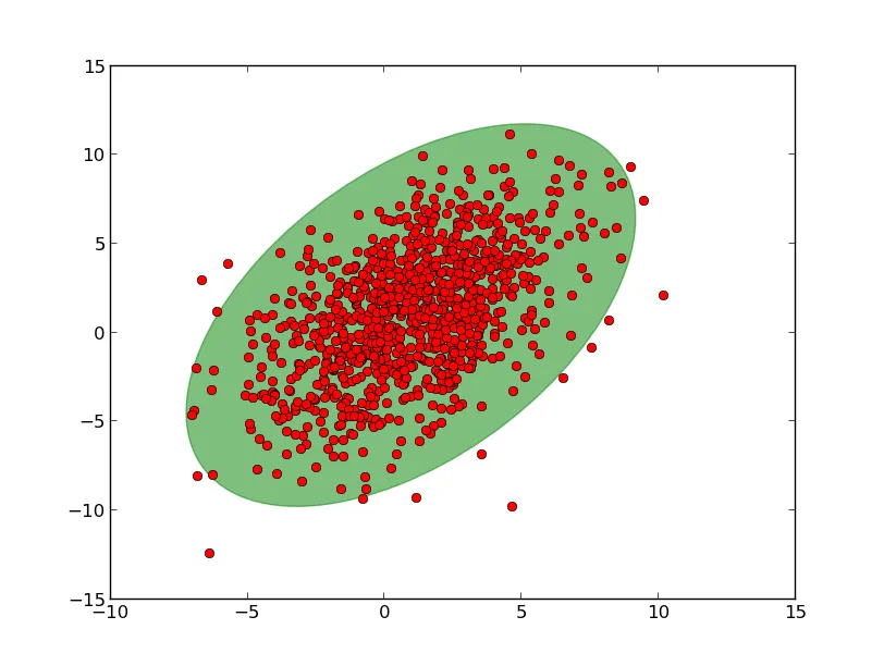
if __name__ == '__main__':
#-- Example usage -----------------------
# Generate some random, correlated data
points = np.random.multivariate_normal(
mean=(1,1), cov=[[0.4, 9],[9, 10]], size=1000
)
# Plot the raw points...
x, y = points.T
plt.plot(x, y, 'ro')
# Plot a transparent 3 standard deviation covariance ellipse
plot_point_cov(points, nstd=3, alpha=0.5, color='green')
plt.show()
nstd,即无论是 68%,90% 还是 95%。 - Srivatsannp.degrees(np.arctan2(*vecs[:,0][::-1])) 计算角度的原理?从这个网站上看到是 arctan(y)/(x),但您使用了 arctan2。 - Srivatsanarctan2 返回完整的角度(可以在任意一个四象限内)。arctan 的输出被限制在第一和第四象限之间(介于-pi / 2和pi / 2之间)。您可能会注意到,arctan 只需要一个参数。因此,它无法区分第一和第四象限中的角度以及第二和第三象限中的类似角度。这是许多其他编程语言共享的惯例,其中 C 定义了它们。 - Joe Kington请参考文章如何绘制协方差误差椭圆。
以下是Python代码实现:
import numpy as np
from scipy.stats import norm, chi2

def cov_ellipse(cov, q=None, nsig=None, **kwargs):
    """
    Parameters
    ----------
    cov : (2, 2) array
        Covariance matrix.
    q : float, optional
        Confidence level, should be in (0, 1)
    nsig : int, optional
        Confidence level in unit of standard deviations.
        E.g. 1 stands for 68.3% and 2 stands for 95.4%.

    Returns
    -------
    width, height, rotation :
         The lengths of two axises and the rotation angle in degree
    for the ellipse.
    """

    if q is not None:
        q = np.asarray(q)
    elif nsig is not None:
        q = 2 * norm.cdf(nsig) - 1
    else:
        raise ValueError('One of `q` and `nsig` should be specified.')
    r2 = chi2.ppf(q, 2)

    val, vec = np.linalg.eigh(cov)
    width, height = 2 * sqrt(val[:, None] * r2)
    rotation = np.degrees(arctan2(*vec[::-1, 0]))

    return width, height, rotation
我稍微修改了上面的一个例子,用于绘制错误或置信区间轮廓。现在我认为它给出了正确的轮廓。
之前它给出了错误的轮廓,因为它将scoreatpercentile方法应用于联合数据集(蓝色 + 红色点),而应该分别应用于每个数据集。
修改后的代码如下:
import numpy
import scipy
import scipy.stats
import matplotlib.pyplot as plt

# generate two normally distributed 2d arrays
x1=numpy.random.multivariate_normal((100,420),[[120,80],[80,80]],400)
x2=numpy.random.multivariate_normal((140,340),[[90,-70],[-70,80]],400)

# fit a KDE to the data
pdf1=scipy.stats.kde.gaussian_kde(x1.T)
pdf2=scipy.stats.kde.gaussian_kde(x2.T)

# create a grid over which we can evaluate pdf
q,w=numpy.meshgrid(range(50,200,10), range(300,500,10))
r1=pdf1([q.flatten(),w.flatten()])
r2=pdf2([q.flatten(),w.flatten()])

# sample the pdf and find the value at the 95th percentile
s1=scipy.stats.scoreatpercentile(pdf1(pdf1.resample(1000)), 5)
s2=scipy.stats.scoreatpercentile(pdf2(pdf2.resample(1000)), 5)

# reshape back to 2d
r1.shape=(20,15)
r2.shape=(20,15)

# plot the contour at the 95th percentile
plt.contour(range(50,200,10), range(300,500,10), r1, [s1],colors='b')
plt.contour(range(50,200,10), range(300,500,10), r2, [s2],colors='r')

# scatter plot the two normal distributions
plt.scatter(x1[:,0],x1[:,1],alpha=0.3)
plt.scatter(x2[:,0],x2[:,1],c='r',alpha=0.3)