使用自定义图像的三维散点图

Question

使用自定义图像的三维散点图

14

我正尝试使用ggplot和ggimage创建一个带有自定义图片的三维散点图。在二维中它可以正常工作：

library(ggplot2)
library(ggimage)
library(rsvg)

set.seed(2017-02-21)
d <- data.frame(x = rnorm(10), y = rnorm(10), z=1:10,
  image = 'https://image.flaticon.com/icons/svg/31/31082.svg'
)

ggplot(d, aes(x, y)) + 
  geom_image(aes(image=image, color=z)) +
  scale_color_gradient(low='burlywood1', high='burlywood4')

我已经尝试了两种方法来创建3D图表：

plotly - 目前无法与geom_image一起使用，但这已排队作为未来请求。
gg3D - 这是一个R包，但我无法使其与自定义图像协调良好。以下是将这些库组合的结果：

library(ggplot2)
library(ggimage)
library(gg3D)

ggplot(d, aes(x=x, y=y, z=z, color=z)) +
  axes_3D() +
  geom_image(aes(image=image, color=z)) +
  scale_color_gradient(low='burlywood1', high='burlywood4')

如果有解决方案，我会接受Python库、JavaScript等任何帮助。

- Adam_G

1

为了吸引更广泛的观众，您可能希望添加标签来表示您愿意考虑的语言/平台。 - Z.Lin

4

即使存在这样的功能，也需要将您的自定义图像转化为3D向量，对于复杂形状来说将会非常棘手。我使用plotly的3D图，但从未尝试过您要寻找的东西。 - Mark

@Adam_G 你可以尝试使用d3.js来实现这个功能。这个d3的例子只是简单的圆形，但它是交互式的，你可以在d3图表中添加自定义形状或者创建它们。不确定是否符合你的需求，但值得一看。 - Rachel Gallen

2个回答

3

这是一个非常粗糙的答案，没有完全解决您的问题，但我认为它是一个好的起点，其他人可能会注意到并达到一个好的解决方案。有一种方法可以在Python中将图像放置为自定义标记。从this AMAZING answer开始，并稍微调整框。
然而，这种解决方案的问题是您的图像没有矢量化（太大无法用作标记）。此外，我没有测试根据色图对其进行着色的方法，因为它实际上不显示为输出：/。这里的基本思想是在创建绘图后用自定义图像替换标记。为了将它们正确地放置在图中，我们按照ImportanceOfBeingErnest的答案检索适当的坐标。

from mpl_toolkits.mplot3d import Axes3D
from mpl_toolkits.mplot3d import proj3d
import matplotlib.pyplot as plt
from matplotlib import offsetbox
import numpy as np

请注意，这里我下载了图像并从本地文件导入它。

import matplotlib.image as mpimg
#
img=mpimg.imread('coffeebean.png')
imgplot = plt.imshow(img)

from PIL import Image
from resizeimage import resizeimage
with open('coffeebean.png', 'r+b') as f:
    with Image.open(f) as image:
        cover = resizeimage.resize_width(image, 20,validate=True)
        cover.save('resizedbean.jpeg', image.format)

img=mpimg.imread('resizedbean.jpeg')
imgplot = plt.imshow(img)

调整大小似乎并不起作用（或者至少我找不到使其起作用的方法）。

xs = [1,1.5,2,2]
ys = [1,2,3,1]
zs = [0,1,2,0]
#c = #I guess copper would be a good colormap here


fig = plt.figure()
ax = fig.add_subplot(111, projection=Axes3D.name)

ax.scatter(xs, ys, zs, marker="None")

# Create a dummy axes to place annotations to
ax2 = fig.add_subplot(111,frame_on=False) 
ax2.axis("off")
ax2.axis([0,1,0,1])

class ImageAnnotations3D():
    def __init__(self, xyz, imgs, ax3d,ax2d):
        self.xyz = xyz
        self.imgs = imgs
        self.ax3d = ax3d
        self.ax2d = ax2d
        self.annot = []
        for s,im in zip(self.xyz, self.imgs):
            x,y = self.proj(s)
            self.annot.append(self.image(im,[x,y]))
        self.lim = self.ax3d.get_w_lims()
        self.rot = self.ax3d.get_proj()
        self.cid = self.ax3d.figure.canvas.mpl_connect("draw_event",self.update)

        self.funcmap = {"button_press_event" : self.ax3d._button_press,
                        "motion_notify_event" : self.ax3d._on_move,
                        "button_release_event" : self.ax3d._button_release}

        self.cfs = [self.ax3d.figure.canvas.mpl_connect(kind, self.cb) \
                        for kind in self.funcmap.keys()]

    def cb(self, event):
        event.inaxes = self.ax3d
        self.funcmap[event.name](event)

    def proj(self, X):
        """ From a 3D point in axes ax1, 
            calculate position in 2D in ax2 """
        x,y,z = X
        x2, y2, _ = proj3d.proj_transform(x,y,z, self.ax3d.get_proj())
        tr = self.ax3d.transData.transform((x2, y2))
        return self.ax2d.transData.inverted().transform(tr)

    def image(self,arr,xy):
        """ Place an image (arr) as annotation at position xy """
        im = offsetbox.OffsetImage(arr, zoom=2)
        im.image.axes = ax
        ab = offsetbox.AnnotationBbox(im, xy, xybox=(0., 0.),
                            xycoords='data', boxcoords="offset points",
                            pad=0.0)
        self.ax2d.add_artist(ab)
        return ab

    def update(self,event):
        if np.any(self.ax3d.get_w_lims() != self.lim) or \
                        np.any(self.ax3d.get_proj() != self.rot):
            self.lim = self.ax3d.get_w_lims()
            self.rot = self.ax3d.get_proj()
            for s,ab in zip(self.xyz, self.annot):
                ab.xy = self.proj(s)



ia = ImageAnnotations3D(np.c_[xs,ys,zs],img,ax, ax2 )

ax.set_xlabel('X Label')
ax.set_ylabel('Y Label')
ax.set_zlabel('Z Label')
plt.show()

你可以看到输出结果远非最佳状态。但是图片位置正确。使用向量化的咖啡豆替代静态咖啡豆可能会有所改善。

附加信息:
尝试使用cv2(每种插值方法)进行调整大小，但没有帮助。
无法在当前工作站上尝试skimage。

您可以尝试以下操作并查看结果。

from skimage.transform import resize
res = resize(img, (20, 20), anti_aliasing=True)

imgplot = plt.imshow(res)

- CAPSLOCK

网页内容由stack overflow 提供, 点击上面的

可以查看英文原文，
原文链接

- Jon Spring · Accepted Answer

这里有一个不太正式的解决方案，它将图像转换为数据框，其中每个像素变成一个体素(?)，然后我们将其发送到plotly中。它基本上可以工作，但需要一些改进来：

1) 更多地调整图像（使用腐蚀步骤？）以排除更多低alpha像素

~~2) 在plotly中使用请求的颜色范围~~

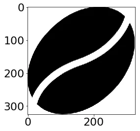
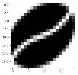
步骤1：导入图像并调整大小，并过滤掉透明或部分透明的像素

library(tidyverse)
library(magick)
sprite_frame <- image_read("coffee-bean-for-a-coffee-break.png") %>% 
  magick::image_resize("20x20") %>% 
  image_raster(tidy = T) %>%
  mutate(alpha = str_sub(col, start = 7) %>% strtoi(base = 16)) %>%
  filter(col != "transparent", 
     alpha > 240)

编辑：如果这个代码块对任何人有用，我会添加结果：

sprite_frame <- 
structure(list(x = c(13L, 14L, 10L, 11L, 12L, 13L, 14L, 15L, 
16L, 17L, 8L, 9L, 10L, 11L, 12L, 13L, 14L, 15L, 16L, 17L, 7L, 
8L, 9L, 10L, 11L, 12L, 13L, 14L, 15L, 16L, 17L, 6L, 7L, 8L, 9L, 
10L, 11L, 12L, 13L, 14L, 15L, 16L, 5L, 6L, 7L, 8L, 9L, 10L, 11L, 
12L, 13L, 14L, 15L, 19L, 4L, 5L, 6L, 7L, 8L, 9L, 10L, 11L, 12L, 
13L, 14L, 19L, 20L, 3L, 4L, 5L, 6L, 7L, 8L, 9L, 10L, 11L, 12L, 
13L, 18L, 19L, 20L, 3L, 4L, 5L, 6L, 7L, 8L, 9L, 10L, 11L, 17L, 
18L, 19L, 2L, 3L, 4L, 5L, 6L, 7L, 8L, 15L, 16L, 17L, 18L, 19L, 
2L, 3L, 4L, 5L, 6L, 13L, 14L, 15L, 16L, 17L, 18L, 19L, 2L, 3L, 
4L, 5L, 11L, 12L, 13L, 14L, 15L, 16L, 17L, 18L, 1L, 2L, 3L, 9L, 
10L, 11L, 12L, 13L, 14L, 15L, 16L, 17L, 18L, 1L, 2L, 7L, 8L, 
9L, 10L, 11L, 12L, 13L, 14L, 15L, 16L, 17L, 2L, 6L, 7L, 8L, 9L, 
10L, 11L, 12L, 13L, 14L, 15L, 16L, 5L, 6L, 7L, 8L, 9L, 10L, 11L, 
12L, 13L, 14L, 15L, 4L, 5L, 6L, 7L, 8L, 9L, 10L, 11L, 12L, 13L, 
14L, 4L, 5L, 6L, 7L, 8L, 9L, 10L, 11L, 12L, 13L, 4L, 5L, 6L, 
7L, 8L, 9L, 10L, 11L, 6L, 7L, 8L), y = c(1L, 1L, 2L, 2L, 2L, 
2L, 2L, 2L, 2L, 2L, 3L, 3L, 3L, 3L, 3L, 3L, 3L, 3L, 3L, 3L, 4L, 
4L, 4L, 4L, 4L, 4L, 4L, 4L, 4L, 4L, 4L, 5L, 5L, 5L, 5L, 5L, 5L, 
5L, 5L, 5L, 5L, 5L, 6L, 6L, 6L, 6L, 6L, 6L, 6L, 6L, 6L, 6L, 6L, 
6L, 7L, 7L, 7L, 7L, 7L, 7L, 7L, 7L, 7L, 7L, 7L, 7L, 7L, 8L, 8L, 
8L, 8L, 8L, 8L, 8L, 8L, 8L, 8L, 8L, 8L, 8L, 8L, 9L, 9L, 9L, 9L, 
9L, 9L, 9L, 9L, 9L, 9L, 9L, 9L, 10L, 10L, 10L, 10L, 10L, 10L, 
10L, 10L, 10L, 10L, 10L, 10L, 11L, 11L, 11L, 11L, 11L, 11L, 11L, 
11L, 11L, 11L, 11L, 11L, 12L, 12L, 12L, 12L, 12L, 12L, 12L, 12L, 
12L, 12L, 12L, 12L, 13L, 13L, 13L, 13L, 13L, 13L, 13L, 13L, 13L, 
13L, 13L, 13L, 13L, 14L, 14L, 14L, 14L, 14L, 14L, 14L, 14L, 14L, 
14L, 14L, 14L, 14L, 15L, 15L, 15L, 15L, 15L, 15L, 15L, 15L, 15L, 
15L, 15L, 15L, 16L, 16L, 16L, 16L, 16L, 16L, 16L, 16L, 16L, 16L, 
16L, 17L, 17L, 17L, 17L, 17L, 17L, 17L, 17L, 17L, 17L, 17L, 18L, 
18L, 18L, 18L, 18L, 18L, 18L, 18L, 18L, 18L, 19L, 19L, 19L, 19L, 
19L, 19L, 19L, 19L, 20L, 20L, 20L), col = c("#000000f6", "#000000fd", 
"#000000f4", "#000000ff", "#000000ff", "#000000ff", "#000000ff", 
"#000000ff", "#000000ff", "#000000f8", "#000000f4", "#000000ff", 
"#000000ff", "#000000ff", "#000000ff", "#000000ff", "#000000ff", 
"#000000ff", "#000000ff", "#000000ff", "#000000ff", "#000000ff", 
"#000000ff", "#000000ff", "#000000ff", "#000000ff", "#000000ff", 
"#000000ff", "#000000ff", "#000000ff", "#000000fd", "#000000ff", 
"#000000ff", "#000000ff", "#000000ff", "#000000ff", "#000000ff", 
"#000000ff", "#000000ff", "#000000ff", "#000000ff", "#000000ff", 
"#000000ff", "#000000ff", "#000000ff", "#000000ff", "#000000ff", 
"#000000ff", "#000000ff", "#000000ff", "#000000ff", "#000000ff", 
"#000000ff", "#000000f9", "#000000ff", "#000000ff", "#000000ff", 
"#000000ff", "#000000ff", "#000000ff", "#000000ff", "#000000ff", 
"#000000ff", "#000000ff", "#000000ff", "#000000ff", "#000000fd", 
"#000000f4", "#000000ff", "#000000ff", "#000000ff", "#000000ff", 
"#000000ff", "#000000ff", "#000000ff", "#000000ff", "#000000ff", 
"#000000fa", "#000000ff", "#000000ff", "#000000f6", "#000000ff", 
"#000000ff", "#000000ff", "#000000ff", "#000000ff", "#000000ff", 
"#000000ff", "#000000ff", "#000000fb", "#000000ff", "#000000ff", 
"#000000ff", "#000000f3", "#000000ff", "#000000ff", "#000000ff", 
"#000000ff", "#000000ff", "#000000ff", "#000000fa", "#000000ff", 
"#000000ff", "#000000ff", "#000000ff", "#000000ff", "#000000ff", 
"#000000ff", "#000000ff", "#000000ff", "#000000f1", "#000000ff", 
"#000000ff", "#000000ff", "#000000ff", "#000000ff", "#000000f3", 
"#000000ff", "#000000ff", "#000000ff", "#000000f6", "#000000f9", 
"#000000ff", "#000000ff", "#000000ff", "#000000ff", "#000000ff", 
"#000000ff", "#000000ff", "#000000f5", "#000000ff", "#000000ff", 
"#000000ff", "#000000ff", "#000000ff", "#000000ff", "#000000ff", 
"#000000ff", "#000000ff", "#000000ff", "#000000ff", "#000000f5", 
"#000000fc", "#000000ff", "#000000fd", "#000000ff", "#000000ff", 
"#000000ff", "#000000ff", "#000000ff", "#000000ff", "#000000ff", 
"#000000ff", "#000000ff", "#000000ff", "#000000f3", "#000000ff", 
"#000000ff", "#000000ff", "#000000ff", "#000000ff", "#000000ff", 
"#000000ff", "#000000ff", "#000000ff", "#000000ff", "#000000ff", 
"#000000ff", "#000000ff", "#000000ff", "#000000ff", "#000000ff", 
"#000000ff", "#000000ff", "#000000ff", "#000000ff", "#000000ff", 
"#000000ff", "#000000ff", "#000000ff", "#000000ff", "#000000ff", 
"#000000ff", "#000000ff", "#000000ff", "#000000ff", "#000000ff", 
"#000000ff", "#000000ff", "#000000ff", "#000000ff", "#000000ff", 
"#000000ff", "#000000ff", "#000000ff", "#000000ff", "#000000ff", 
"#000000ff", "#000000f5", "#000000f8", "#000000ff", "#000000ff", 
"#000000ff", "#000000ff", "#000000ff", "#000000ff", "#000000f4", 
"#000000f1", "#000000fe", "#000000f7"), alpha = c(246L, 253L, 
244L, 255L, 255L, 255L, 255L, 255L, 255L, 248L, 244L, 255L, 255L, 
255L, 255L, 255L, 255L, 255L, 255L, 255L, 255L, 255L, 255L, 255L, 
255L, 255L, 255L, 255L, 255L, 255L, 253L, 255L, 255L, 255L, 255L, 
255L, 255L, 255L, 255L, 255L, 255L, 255L, 255L, 255L, 255L, 255L, 
255L, 255L, 255L, 255L, 255L, 255L, 255L, 249L, 255L, 255L, 255L, 
255L, 255L, 255L, 255L, 255L, 255L, 255L, 255L, 255L, 253L, 244L, 
255L, 255L, 255L, 255L, 255L, 255L, 255L, 255L, 255L, 250L, 255L, 
255L, 246L, 255L, 255L, 255L, 255L, 255L, 255L, 255L, 255L, 251L, 
255L, 255L, 255L, 243L, 255L, 255L, 255L, 255L, 255L, 255L, 250L, 
255L, 255L, 255L, 255L, 255L, 255L, 255L, 255L, 255L, 241L, 255L, 
255L, 255L, 255L, 255L, 243L, 255L, 255L, 255L, 246L, 249L, 255L, 
255L, 255L, 255L, 255L, 255L, 255L, 245L, 255L, 255L, 255L, 255L, 
255L, 255L, 255L, 255L, 255L, 255L, 255L, 245L, 252L, 255L, 253L, 
255L, 255L, 255L, 255L, 255L, 255L, 255L, 255L, 255L, 255L, 243L, 
255L, 255L, 255L, 255L, 255L, 255L, 255L, 255L, 255L, 255L, 255L, 
255L, 255L, 255L, 255L, 255L, 255L, 255L, 255L, 255L, 255L, 255L, 
255L, 255L, 255L, 255L, 255L, 255L, 255L, 255L, 255L, 255L, 255L, 
255L, 255L, 255L, 255L, 255L, 255L, 255L, 255L, 255L, 245L, 248L, 
255L, 255L, 255L, 255L, 255L, 255L, 244L, 241L, 254L, 247L)), row.names = c(NA, 
-210L), class = "data.frame")

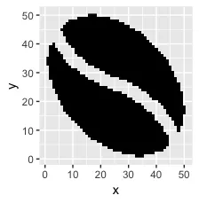
以下是它的样子：

ggplot(sprite_frame, aes(x,y, fill = col)) + 
  geom_raster() + 
  guides(fill = F) +
  scale_fill_identity()

第二步：将这些像素转换为体素

pixels_per_image <- nrow(sprite_frame)
scale <- 1/40  # How big should a pixel be in coordinate space?

set.seed(2017-02-21)
d <- data.frame(x = rnorm(10), y = rnorm(10), z=1:10)
d2 <- d %>%
  mutate(copies = pixels_per_image) %>%
  uncount(copies) %>%
  mutate(x_sprite = sprite_frame$x*scale + x,
         y_sprite = sprite_frame$y*scale + y,
         col = rep(sprite_frame$col, nrow(d)))

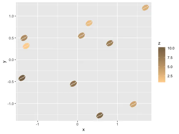
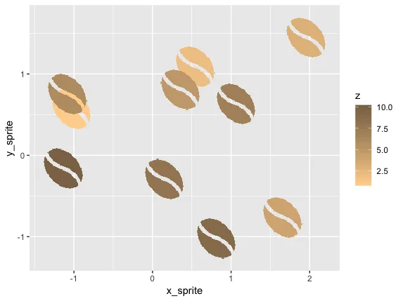
我们可以使用ggplot在二维空间中绘制它：

ggplot(d2, aes(x_sprite, y_sprite, z = z, alpha = col, fill = z)) + 
  geom_tile(width = scale, height = scale) + 
  guides(alpha = F) +
  scale_fill_gradient(low='burlywood1', high='burlywood4')

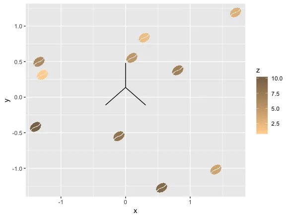
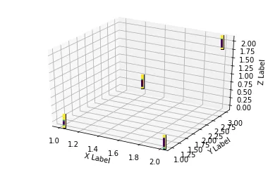
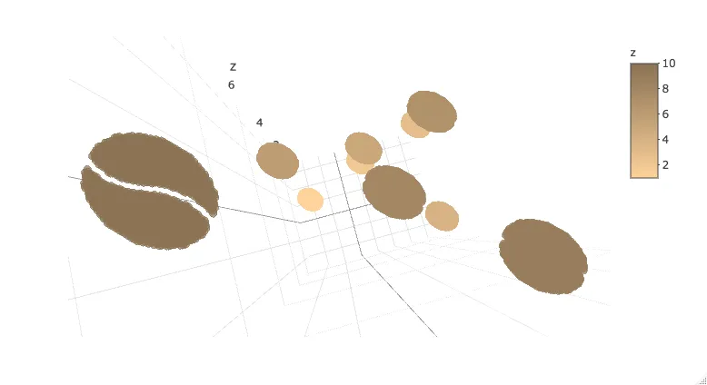
或者将其导入到Plotly中。请注意，目前Plotly 3D散点图不支持可变透明度，因此在缩放到一个精灵时，图像会显示为实心椭圆。

library(plotly)
plot_ly(d2, x = ~x_sprite, y = ~y_sprite, z = ~z, 
    size = scale, color = ~z, colors = c("#FFD39B", "#8B7355")) %>%
    add_markers()

编辑：尝试使用plotly的mesh3d方法

另一种方法似乎是将SVG图形转换为plotly中mesh3d表面的坐标。

我最初尝试这样做的方法非常繁琐：

在Inkscape中加载SVG并使用“flatten beziers”选项来近似不带bezier曲线的形状。
导出SVG并祈祷文件具有原始坐标。我对SVG还不太熟悉，看起来输出通常可以是绝对和相对点的混合体。在此情况下更加复杂，因为该字形有两个断开的部分。
将坐标重新格式化为数据框以便使用ggplot2或plotly进行绘制。

例如，以下坐标表示半个豆子，我们可以通过变换得到另外一半：

library(dplyr)
half_bean <- read.table(
  header = T,
  stringsAsFactors = F,
  text = "x y
  153.714 159.412 
  95.490016 186.286 
  54.982625 216.85 
  28.976672 247.7425 
  14.257 275.602 
  0.49742188 229.14067 
  5.610375 175.89737 
  28.738141 120.85839 
  69.023 69.01 
  128.24827 24.564609 
  190.72412 2.382875 
  249.14492 3.7247031 
  274.55165 13.610674 
  296.205 29.85 
  296.4 30.064 
  283.67119 58.138937 
  258.36 93.03325 
  216.39731 128.77994 
  153.714 159.412"
) %>%
  mutate(z = 0)

other_half <- half_bean %>%
  mutate(x = 330 - x,
         y = 330 - y,
         z = z)

ggplot() + coord_equal() +
  geom_path(data = half_bean, aes(x,y)) +
  geom_path(data = other_half, aes(x,y))

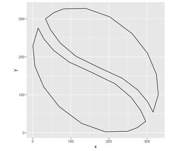
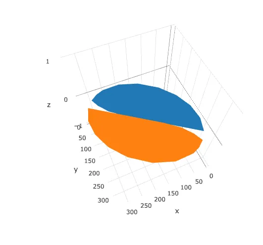
虽然在ggplot中看起来不错，但我在plotly中遇到了显示凹形部分的问题：

library(plotly)
plot_ly(type = 'mesh3d',
        split = c(rep(1, 19), rep(2, 19)),
             x = c(half_bean$x, other_half$x),
             y = c(half_bean$y, other_half$y),
             z = c(half_bean$z, other_half$z)
)