在Matplotlib中找到两条曲线之间的面积（使用fill_between函数）

Question

我有两条曲线的x和y值的列表，它们都具有奇怪的形状，并且我没有任何一个曲线的函数。我需要做两件事:

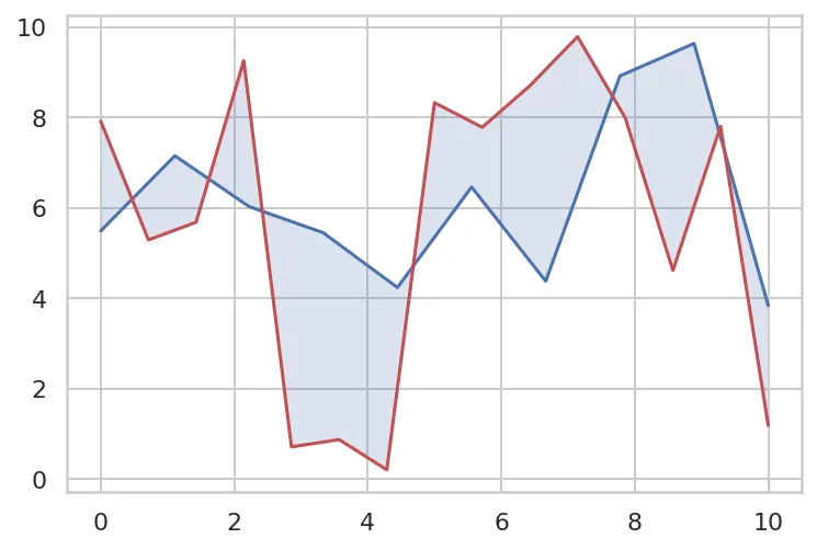
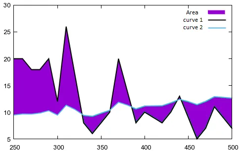
1. 绘制这些曲线并填充它们之间的阴影区域，就像下面的图片一样。
2. 找到这些被填充的曲线之间的阴影区域的总面积。

我能够使用matplotlib中的fill_between和fill_betweenx绘制并填充这些曲线之间的区域，但我不知道如何计算它们之间的确切面积，特别是因为我没有这些曲线的任何函数。
有什么想法吗？

我已经搜索了所有地方，但找不到简单的解决方法。我非常绝望，所以非常感谢任何帮助。

非常感谢！

---

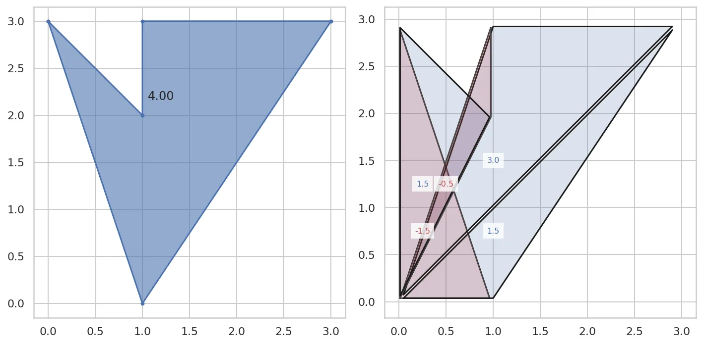
编辑:供以后参考(如果有人遇到同样的问题),这是我解决的方法:连接每条曲线的第一个和最后一个节点/点,得到一个大的奇怪形状的多边形，然后使用shapely自动计算多边形的面积，这是曲线之间的确切面积，无论它们朝哪个方向或者有多么非线性。效果惊人！ :)

这是我的代码:

from shapely.geometry import Polygon

x_y_curve1 = [(0.121,0.232),(2.898,4.554),(7.865,9.987)] #these are your points for curve 1 (I just put some random numbers)
x_y_curve2 = [(1.221,1.232),(3.898,5.554),(8.865,7.987)] #these are your points for curve 2 (I just put some random numbers)

polygon_points = [] #creates a empty list where we will append the points to create the polygon

for xyvalue in x_y_curve1:
    polygon_points.append([xyvalue[0],xyvalue[1]]) #append all xy points for curve 1

for xyvalue in x_y_curve2[::-1]:
    polygon_points.append([xyvalue[0],xyvalue[1]]) #append all xy points for curve 2 in the reverse order (from last point to first point)

for xyvalue in x_y_curve1[0:1]:
    polygon_points.append([xyvalue[0],xyvalue[1]]) #append the first point in curve 1 again, to it "closes" the polygon

polygon = Polygon(polygon_points)
area = polygon.area
print(area)

编辑 2：感谢回答。就像 Kyle 解释的那样，这只适用于正值。如果您的曲线低于0（这不是我的情况，如示例图表所示），那么您将不得不使用绝对数值。

- F4R

---

我非常喜欢那个答案，但需要注意的是该区域在第一条线的上方和下方被取消。例如，考虑一个简单的蝴蝶结： coords = [(0,0),(0,1),(1,0),(1,1),(0,0)] Polygon(coords).area 这将给出一个面积为0的结果，尽管它实际上不是0。 - Kyle Barron

相反，如果你想要绝对值，计算正负多边形的数量，你应该遵循这个答案（https://gis.stackexchange.com/a/243498），然后计算列表中每个多边形的面积。 - Kyle Barron

是的，我认为楼主的方法只是从另一个区域中减去了一个区域...这是我从代码中得到的结果。因此，需要添加Kyle的内容。 - SGhaleb

Answer 1

如果两条曲线不相交，面积计算很简单：就是上面提到的梯形。如果它们相交了，则在 x[i] 和 x[i+1] 之间创建两个三角形，并应将两个三角形的面积相加。如果您想直接计算，请分别处理这两种情况。下面是一个基本的工作示例来解决您的问题。首先，我将从一些虚假数据开始：

#!/usr/bin/python
import numpy as np

# let us generate fake test data
x = np.arange(10)
y1 = np.random.rand(10) * 20
y2 = np.random.rand(10) * 20

现在，进入主要的代码。根据您的图表, 看起来您定义了y1和y2在相同的X点。接下来我们定义:

z = y1-y2
dx = x[1:] - x[:-1]
cross_test = np.sign(z[:-1] * z[1:])

当两个图形相交时，cross_test会变为负值。在这些点上，我们想计算交叉点的x坐标。为了简单起见，我将计算y所有线段的交点的x坐标。对于两条曲线不相交的地方，它们将是无用的值，我们不会在任何地方使用它们。这只是使代码更容易理解。

假设您在x1和x2处有z1和z2，则我们正在解决z = 0的x0：

# (z2 - z1)/(x2 - x1) = (z0 - z1) / (x0 - x1) = -z1/(x0 - x1)
# x0 = x1 - (x2 - x1) / (z2 - z1) * z1
x_intersect = x[:-1] - dx / (z[1:] - z[:-1]) * z[:-1]
dx_intersect = - dx / (z[1:] - z[:-1]) * z[:-1]

当曲线不相交时，面积可以简单地表示为：

areas_pos = abs(z[:-1] + z[1:]) * 0.5 * dx # signs of both z are same

当它们相交时，我们添加两个三角形的面积：

areas_neg = 0.5 * dx_intersect * abs(z[:-1]) + 0.5 * (dx - dx_intersect) * abs(z[1:])

现在需要选择每个块x[i]到x[i+1]中的区域，我使用np.where实现：

areas = np.where(cross_test < 0, areas_neg, areas_pos)
total_area = np.sum(areas)

这就是您想要的答案。正如上面所指出的，如果两个y图在不同的x点上定义，这将变得更加复杂。如果您想测试此内容，可以简单地绘制它（在我的测试中，y范围将为-20至20）。

negatives = np.where(cross_test < 0)
positives = np.where(cross_test >= 0)
plot(x, y1)
plot(x, y2)
plot(x, z)
plt.vlines(x_intersect[negatives], -20, 20)

- VBB

Answer 2

将你的两个曲线定义为函数f和g，这些函数是由线段组成的，例如在x1和x2之间，f(x)=f(x1)+((x-x1)/(x2-x1))*(f(x2)-f(x1))。定义h(x)=abs(g(x)-f(x))。然后使用scipy.integrate.quad来对h进行积分。这样就不需要担心交点了。它会自动执行ch41rmn建议的“梯形求和”。

- JulienD

---

@JulieD 是否有一种方法可以在不能定义函数但有一组点的情况下实现此操作？我的一个函数是直线，但另一个函数只是我连接的点。有什么想法吗？ - guy

@guy 是的，就像在OP的例子中一样，您总是可以定义一个在集合中点之间以线性方式定义函数的函数，即定义一个函数，它接受一个 x ，找到该集合中紧靠其前后的点（x1，x2），并返回上面的 f(x)。 - JulienD

谢谢您的回复，我尝试了但无法实现。您能提供一个例子吗？也许我可以发起一个新问题，这样您就可以回答那个问题，我可以通过那种方式接受它。请告诉我。谢谢。 - guy

@guy 如果您打算发布一篇新帖子并展示一些尝试，请务必这样做。 - JulienD

这个过程的名称存在吗？或者你知道一些数学参考资料吗？ - helmi

@helmi 这只是一个线段的数学定义，然后是两个任意函数之间的差异。根据其定义，h 是在任何点 x 给出差异的函数，因此如果你对其进行积分，你将得到区间内曲线之间的面积。任何数学教科书都有这些内容，没有特定的名称（但将其扩展到 N 维）。 - JulienD

Answer 3

你的数据集在某种意义上非常"完美"，因为两组数据共享相同的x坐标集。因此，你可以使用一系列梯形来计算面积。

例如，将这两个函数定义为f（x）和g（x），然后在x的任何两个连续点之间，你有四个数据点：

(x1, f(x1))-->(x2, f(x2))
(x1, g(x1))-->(x2, g(x2))

然后，这个梯形的面积是：

A(x1-->x2) = ( f(x1)-g(x1) + f(x2)-g(x2) ) * (x2-x1)/2                         (1)

一个问题出现了，方程式 (1) 只适用于简单连通区域，即该区域内不得有交叉：

|\             |\/|
|_|     vs     |/\|

交点两侧的面积必须分别计算。您需要检查数据以找到所有交点，然后将它们的坐标插入到坐标列表中。必须保持正确的x顺序。然后，您可以循环遍历简单连通区域列表，并获得梯形面积之和。

编辑：如果两个列表的x坐标不同，您可以构造三角形。例如：

.____.
|   / \
|  /   \
| /     \
|/       \
._________.

在处理三角形时，我们需要避免它们之间的重叠，因此您需要再次查找交点并将其插入到有序列表中。可以使用勾股定理计算三角形的每条边长，使用海伦公式计算三角形的面积。

- ch41rmn

Answer 4

pypi库similaritymeasures中的area_between_two_curves函数（2018年发布）可能会给您所需的内容。我在我的电脑上尝试了一个简单的例子，比较了一个函数和一个常数值之间的面积，并且与Excel非常接近（误差不超过2%）。不确定为什么它没有给我100%的匹配，也许是我做错了什么。但这是值得考虑的。

- GivenX

Answer 5

我有同样的问题。下面的答案是基于问题作者的尝试。然而，shapely不会直接给出紫色多边形的面积。您需要编辑代码将其分解为其组成多边形，然后获取每个多边形的面积。之后，您只需将它们相加即可。

考虑下面的线条： 两条线之间的区域 以下是代码： 示例两条线 如果您运行以下代码，则会得到零面积，因为它将顺时针面积减去逆时针面积：

from shapely.geometry import Polygon

x_y_curve1 = [(1,1),(2,1),(3,3),(4,3)] #these are your points for curve 1 
x_y_curve2 = [(1,3),(2,3),(3,1),(4,1)] #these are your points for curve 2 

polygon_points = [] #creates a empty list where we will append the points to create the polygon

for xyvalue in x_y_curve1:
    polygon_points.append([xyvalue[0],xyvalue[1]]) #append all xy points for curve 1

for xyvalue in x_y_curve2[::-1]:
    polygon_points.append([xyvalue[0],xyvalue[1]]) #append all xy points for curve 2 in the reverse order (from last point to first point)

for xyvalue in x_y_curve1[0:1]:
    polygon_points.append([xyvalue[0],xyvalue[1]]) #append the first point in curve 1 again, to it "closes" the polygon

polygon = Polygon(polygon_points)
area = polygon.area
print(area)

因此，解决方案是根据线段相交的位置将多边形分割成较小的部分。然后使用for循环将它们加起来：

from shapely.geometry import Polygon

x_y_curve1 = [(1,1),(2,1),(3,3),(4,3)] #these are your points for curve 1 
x_y_curve2 = [(1,3),(2,3),(3,1),(4,1)] #these are your points for curve 2 

polygon_points = [] #creates a empty list where we will append the points to create the polygon

for xyvalue in x_y_curve1:
    polygon_points.append([xyvalue[0],xyvalue[1]]) #append all xy points for curve 1

for xyvalue in x_y_curve2[::-1]:
    polygon_points.append([xyvalue[0],xyvalue[1]]) #append all xy points for curve 2 in the reverse order (from last point to first point)

for xyvalue in x_y_curve1[0:1]:
    polygon_points.append([xyvalue[0],xyvalue[1]]) #append the first point in curve 1 again, to it "closes" the polygon

polygon = Polygon(polygon_points)
area = polygon.area

x,y = polygon.exterior.xy
    # original data
ls = LineString(np.c_[x, y])
    # closed, non-simple
lr = LineString(ls.coords[:] + ls.coords[0:1])
lr.is_simple  # False
mls = unary_union(lr)
mls.geom_type  # MultiLineString'

Area_cal =[]

for polygon in polygonize(mls):
    Area_cal.append(polygon.area)
    Area_poly = (np.asarray(Area_cal).sum())
print(Area_poly)

- Rubbani Boris

---

这是一个有趣的方法，但似乎需要几个导入行：

from shapely.geometry import LineString; from shapely.ops import unary_union; 不确定 polygonize，也许是从 GDAL？

- CreekGeek

@Creek 从 shapely.ops 导入 unary_union、polygonize - SGhaleb

Answer 6

一个简单的多边形面积应用（参见鞋带公式）可以实现超级简单、快速和矢量化的计算：

def area(p):
    # for p: 2D vertices of a polygon:
    # area = 1/2 abs(sum(p0 ^ p1 + p1 ^ p2 + ... + pn-1 ^ p0))
    # where ^ is the cross product
    return np.abs(np.cross(p, np.roll(p, 1, axis=0)).sum()) / 2

计算两条曲线之间的面积。在这个例子中，我们甚至没有匹配的x坐标!

np.random.seed(0)
n0 = 10
n1 = 15
xy0 = np.c_[np.linspace(0, 10, n0), np.random.uniform(0, 10, n0)]
xy1 = np.c_[np.linspace(0, 10, n1), np.random.uniform(0, 10, n1)]

p = np.r_[xy0, xy1[::-1]]
>>> area(p)
4.9786...

情节：

plt.plot(*xy0.T, 'b-')
plt.plot(*xy1.T, 'r-')
p = np.r_[xy0, xy1[::-1]]
plt.fill(*p.T, alpha=.2)

速度

对于具有100万个点的两条曲线：

n = 1_000_000
xy0 = np.c_[np.linspace(0, 10, n), np.random.uniform(0, 10, n)]
xy1 = np.c_[np.linspace(0, 10, n), np.random.uniform(0, 10, n)]

%timeit area(np.r_[xy0, xy1[::-1]])
# 42.9 ms ± 140 µs per loop (mean ± std. dev. of 7 runs, 10 loops each)

计算多边形面积的简单可视化

# say:
p = np.array([[0, 3], [1, 0], [3, 3], [1, 3], [1, 2]])

p_closed = np.r_[p, p[:1]]
fig, axes = plt.subplots(ncols=2, figsize=(10, 5), subplot_kw=dict(box_aspect=1), sharex=True)
ax = axes[0]
ax.set_aspect('equal')
ax.plot(*p_closed.T, '.-')
ax.fill(*p_closed.T, alpha=0.6)
center = p.mean(0)
txtkwargs = dict(ha='center', va='center')
ax.text(*center, f'{area(p):.2f}', **txtkwargs)
ax = axes[1]
ax.set_aspect('equal')
for a, b in zip(p_closed, p_closed[1:]):
    ar = 1/2 * np.cross(a, b)
    pos = ar >= 0
    tri = np.c_[(0,0), a, b, (0,0)].T
    # shrink a bit to make individual triangles easier to visually identify
    center = tri.mean(0)
    tri = (tri - center)*0.95 + center
    c = 'b' if pos else 'r'
    ax.plot(*tri.T, 'k')
    ax.fill(*tri.T, c, alpha=0.2, zorder=2 - pos)
    t = ax.text(*center, f'{ar:.1f}', color=c, fontsize=8, **txtkwargs)
    t.set_bbox(dict(facecolor='white', alpha=0.8, edgecolor='none'))

plt.tight_layout()

- Pierre D

Answer 7

一种优雅的方法是通过在shapely.geometry包中结合fill_between()函数和Polygon函数来实现。 fill_between()返回一个PolyCollection对象，您可以从中获取每个多边形的路径。好处是您甚至可以分别计算y2>y1和y2<y1的面积。

import numpy as np
import matplotlib.pyplot as plt
from shapely.geometry import Polygon

n = 10
y1 = np.random.uniform(0, 10, n)
y2 = np.random.uniform(0, 10, n)

fig, ax = plt.subplots()
poly_collect = ax.fill_between(y1, y2)
paths = poly_collect.get_paths()
area = 0
for path in paths:
    poly = Polygon(path.vertices)
    area += poly.area

- Qing-Long LU