Python中轮廓选定的网格区域外边缘的方法

Question

I have the following code:

import numpy as np
import matplotlib.pyplot as plt

x = np.linspace(-np.pi/2, np.pi/2, 30)
y = np.linspace(-np.pi/2, np.pi/2, 30)
x,y = np.meshgrid(x,y)

z = np.sin(x**2+y**2)[:-1,:-1]

fig,ax = plt.subplots()
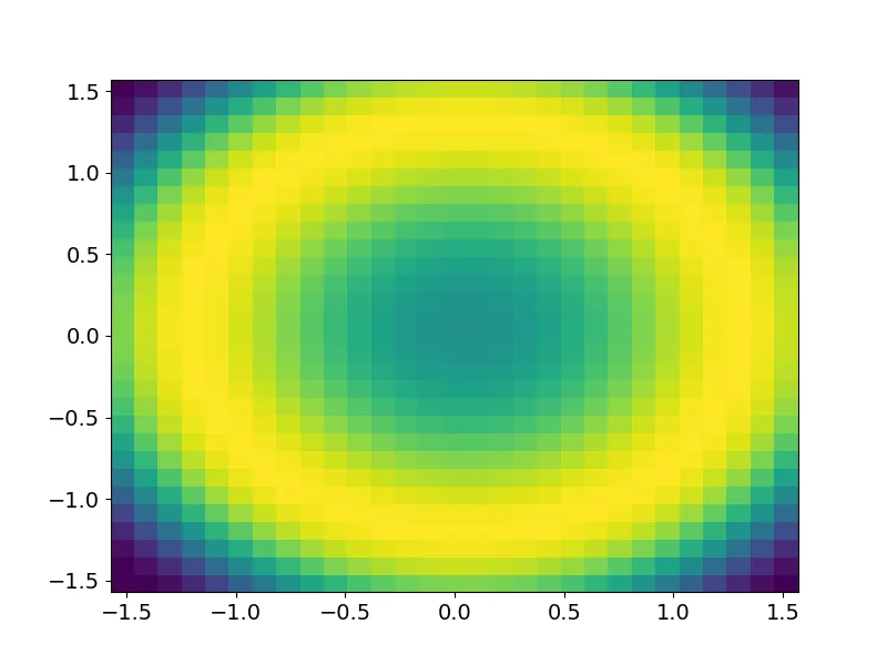
ax.pcolormesh(x,y,z)

这将得到以下图片：

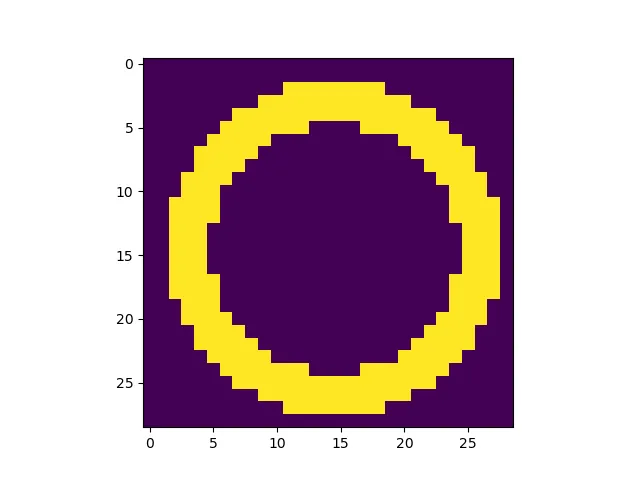
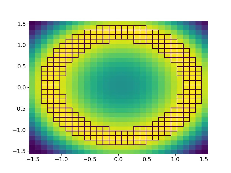
现在假设我想突出显示某些网格框的边缘：

highlight = (z > 0.9)

我可以使用轮廓函数，但这会导致“平滑”的轮廓。我只想突出显示区域的边缘，沿着网格框的边缘。

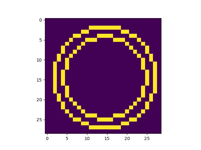
我最接近的方法是添加类似以下内容：

highlight = np.ma.masked_less(highlight, 1)

ax.pcolormesh(x, y, highlight, facecolor = 'None', edgecolors = 'w')

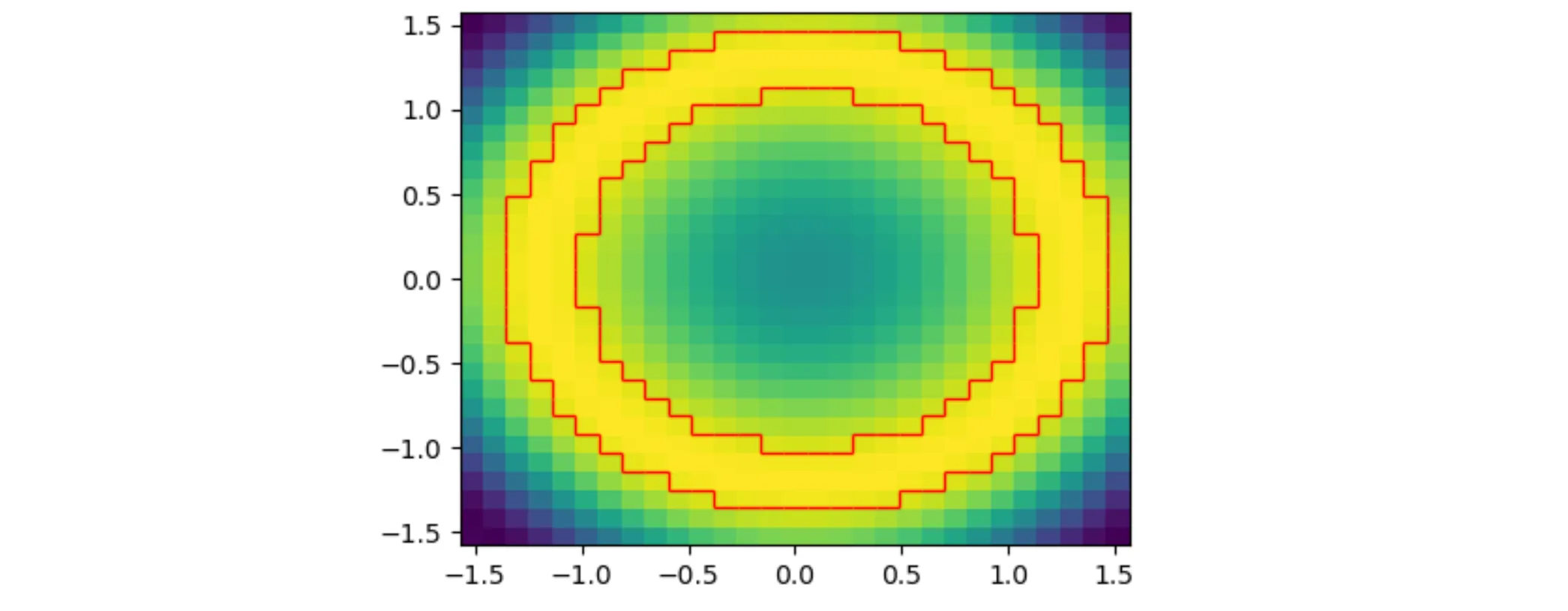
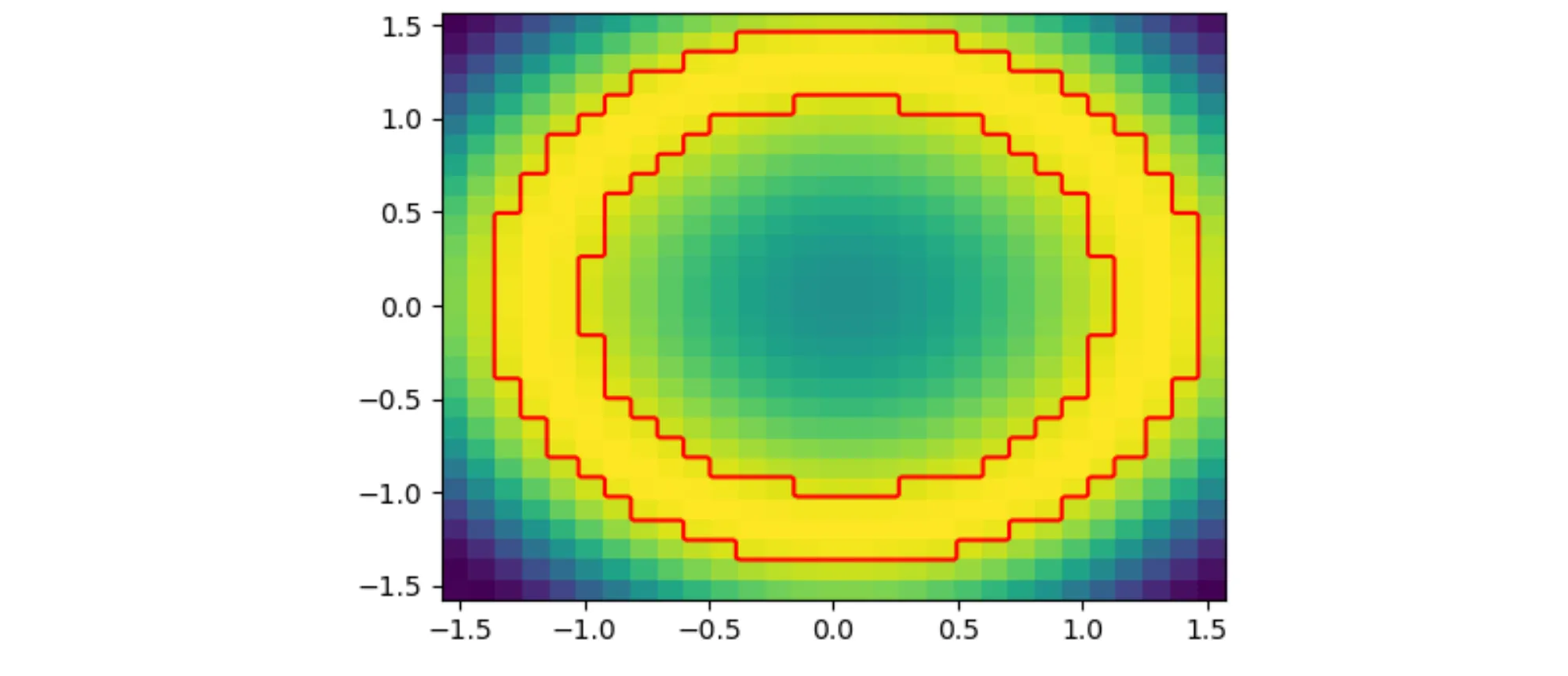
这给出了这个图形： 这很接近，但我真正想要的是只突出显示“甜甜圈”的外边缘和内边缘。

因此，我正在寻找一些轮廓和pcolormesh函数的混合体 - 跟随某个值的轮廓，但是步进网格单元而不是点对点连接。这有意义吗？

附注：在pcolormesh参数中，我有edgecolors='w'，但边缘仍然变为蓝色。发生了什么事？

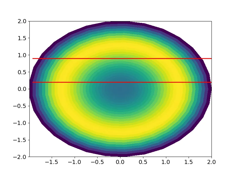
编辑：JohanC最初的答案使用add_iso_line()适用于所提出的问题。然而，我使用的实际数据是非常不规则的x，y网格，不能转换为1D（如add_iso_line()所需）。

我正在使用已从极坐标（rho，phi）转换为笛卡尔（x，y）的数据。 JohanC提出的2D解决方案似乎不适用于以下情况：

import numpy as np
import matplotlib.pyplot as plt
from scipy import ndimage

def pol2cart(rho, phi):
    x = rho * np.cos(phi)
    y = rho * np.sin(phi)
    return(x, y)

phi = np.linspace(0,2*np.pi,30)
rho = np.linspace(0,2,30)

pp, rr = np.meshgrid(phi,rho)

xx,yy = pol2cart(rr, pp)

z = np.sin(xx**2 + yy**2)

scale = 5
zz = ndimage.zoom(z, scale, order=0)

fig,ax = plt.subplots()
ax.pcolormesh(xx,yy,z[:-1, :-1])

xlim = ax.get_xlim()
ylim = ax.get_ylim()
xmin, xmax = xx.min(), xx.max()
ymin, ymax = yy.min(), yy.max()
ax.contour(np.linspace(xmin,xmax, zz.shape[1]) + (xmax-xmin)/z.shape[1]/2,
           np.linspace(ymin,ymax, zz.shape[0]) + (ymax-ymin)/z.shape[0]/2,
           np.where(zz < 0.9, 0, 1), levels=[0.5], colors='red')
ax.set_xlim(*xlim)
ax.set_ylim(*ylim)

- hm8

---

是的，这是一个清晰且非常有用的问题。 - mathfux

z[z>0.9] = 0 或 z[z>0.9] = 1 来改变值，使它们不同。请注意，pyplot 自动分配了一个颜色映射。您可能想使用灰度颜色映射。或者您可能只想使用 cv2.imshow() 在灰度中查看它。然后，您可以将其转换为 3 个通道，并使强调红色 z1=cv2.merge([z,z,z])，然后 z1[z>0.9]=(255,255,255)。 - fmw42

Answer 1

这篇文章展示了一种绘制这样线条的方法。由于要适应当前的pcolormesh并不直接，以下代码演示了可能的调整方式。 请注意，x和y的2d版本已被重命名，因为需要1d版本来绘制线段。

import numpy as np
import matplotlib.pyplot as plt
from matplotlib.collections import LineCollection

x = np.linspace(-np.pi / 2, np.pi / 2, 30)
y = np.linspace(-np.pi / 2, np.pi / 2, 30)
xx, yy = np.meshgrid(x, y)

z = np.sin(xx ** 2 + yy ** 2)[:-1, :-1]

fig, ax = plt.subplots()
ax.pcolormesh(x, y, z)

def add_iso_line(ax, value, color):
    v = np.diff(z > value, axis=1)
    h = np.diff(z > value, axis=0)

    l = np.argwhere(v.T)
    vlines = np.array(list(zip(np.stack((x[l[:, 0] + 1], y[l[:, 1]])).T,
                               np.stack((x[l[:, 0] + 1], y[l[:, 1] + 1])).T)))
    l = np.argwhere(h.T)
    hlines = np.array(list(zip(np.stack((x[l[:, 0]], y[l[:, 1] + 1])).T,
                               np.stack((x[l[:, 0] + 1], y[l[:, 1] + 1])).T)))
    lines = np.vstack((vlines, hlines))
    ax.add_collection(LineCollection(lines, lw=1, colors=color))

add_iso_line(ax, 0.9, 'r')
plt.show()

这是第二个答案的改编版本，可以仅使用2D数组来实现：

import numpy as np
import matplotlib.pyplot as plt
from matplotlib.collections import LineCollection
from scipy import ndimage

x = np.linspace(-np.pi / 2, np.pi / 2, 30)
y = np.linspace(-np.pi / 2, np.pi / 2, 30)
x, y = np.meshgrid(x, y)

z = np.sin(x ** 2 + y ** 2)

scale = 5
zz = ndimage.zoom(z, scale, order=0)

fig, ax = plt.subplots()
ax.pcolormesh(x, y,  z[:-1, :-1] )
xlim = ax.get_xlim()
ylim = ax.get_ylim()
xmin, xmax = x.min(), x.max()
ymin, ymax = y.min(), y.max()
ax.contour(np.linspace(xmin,xmax, zz.shape[1]) + (xmax-xmin)/z.shape[1]/2,
           np.linspace(ymin,ymax, zz.shape[0]) + (ymax-ymin)/z.shape[0]/2,
           np.where(zz < 0.9, 0, 1), levels=[0.5], colors='red')
ax.set_xlim(*xlim)
ax.set_ylim(*ylim)
plt.show()

- JohanC

---

好的，这回答了所提出的问题。然而，我想我简化得太多了。在我实际处理的数据集中，x和y不是在一个常规网格上 - 我不能将它们变成1-D。我应该发一个新问题吗？ - hm8

你可以从2D版本中提取1D版本。类似这样：x1d = x[0,:] 和 y1d = y[:,0]。如果需要，可以继续提问或添加新问题。 - JohanC

提出的二维解决方案对我的情况不起作用。我已经使用新的示例更新了原始问题。 - hm8

Answer 2

我将尝试对add_iso_line方法进行重构，以使其更清晰并开放优化。因此，首先需要完成必须的部分：

import numpy as np
import matplotlib.pyplot as plt
from matplotlib.collections import LineCollection

x = np.linspace(-np.pi/2, np.pi/2, 30)
y = np.linspace(-np.pi/2, np.pi/2, 30)
x, y = np.meshgrid(x,y)
z = np.sin(x**2+y**2)[:-1,:-1]

fig, ax = plt.subplots()
ax.pcolormesh(x,y,z)
xlim, ylim = ax.get_xlim(), ax.get_ylim()
highlight = (z > 0.9)

现在，highlight是一个二进制数组，看起来像这样： 之后，我们可以提取True单元格的索引，查找False邻域并确定“红色”线的位置。我不太熟悉以向量化的方式执行此操作（例如在add_iso_line方法中），因此只使用简单循环：

lines = []
cells = zip(*np.where(highlight))
for x, y in cells:
    if x == 0 or highlight[x - 1, y] == 0: lines.append(([x, y], [x, y + 1]))
    if x == highlight.shape[0] or highlight[x + 1, y] == 0: lines.append(([x + 1, y], [x + 1, y + 1]))
    if y == 0 or highlight[x, y - 1] == 0: lines.append(([x, y], [x + 1, y]))
    if y == highlight.shape[1] or highlight[x, y + 1] == 0: lines.append(([x, y + 1], [x + 1, y + 1]))

最后，我会调整线条的大小和居中坐标以适应 pcolormesh。

lines = (np.array(lines) / highlight.shape - [0.5, 0.5]) * [xlim[1] - xlim[0], ylim[1] - ylim[0]]
ax.add_collection(LineCollection(lines, colors='r'))
plt.show()

总之，这与JohanC的解决方案非常相似，并且通常较慢。幸运的是，我们可以通过仅使用python-opencv包提取轮廓来显着减少cells的数量：

import cv2
highlight = highlight.astype(np.uint8)
contours, hierarchy = cv2.findContours(highlight, cv2.RETR_TREE, cv2.CHAIN_APPROX_NONE)
cells = np.vstack(contours).squeeze()

这是细胞被检查的示意图：

- mathfux