如何在Python的Matplotlib线条上绘制外边缘的轮廓？

Question

我试图在 `networkx` 的边缘上绘制一个轮廓线 (`linestyle=":"`)。我似乎无法弄清如何对 `matplotlib` 的 `patch` 对象进行操作以绘制这些 "edges" 的轮廓线。如果这不可能，有人知道如何单独获取线数据并使用 `ax.plot(x, y, linestyle=":")` 来完成此操作吗？

import networkx as nx
import numpy as np
from collections import *

# Graph data
G = {'y1': OrderedDict([('y2', OrderedDict([('weight', 0.8688325076457851)])), (1, OrderedDict([('weight', 0.13116749235421485)]))]), 'y2': OrderedDict([('y3', OrderedDict([('weight', 0.29660515972204304)])), ('y4', OrderedDict([('weight', 0.703394840277957)]))]), 'y3': OrderedDict([(4, OrderedDict([('weight', 0.2858185316736193)])), ('y5', OrderedDict([('weight', 0.7141814683263807)]))]), 4: OrderedDict(), 'input': OrderedDict([('y1', OrderedDict([('weight', 1.0)]))]), 'y4': OrderedDict([(3, OrderedDict([('weight', 0.27847763084646443)])), (5, OrderedDict([('weight', 0.7215223691535356)]))]), 3: OrderedDict(), 5: OrderedDict(), 'y5': OrderedDict([(6, OrderedDict([('weight', 0.5733512797415756)])), (2, OrderedDict([('weight', 0.4266487202584244)]))]), 6: OrderedDict(), 1: OrderedDict(), 2: OrderedDict()}
G = nx.from_dict_of_dicts(G)
G_scaffold = {'input': OrderedDict([('y1', OrderedDict())]), 'y1': OrderedDict([('y2', OrderedDict()), (1, OrderedDict())]), 'y2': OrderedDict([('y3', OrderedDict()), ('y4', OrderedDict())]), 1: OrderedDict(), 'y3': OrderedDict([(4, OrderedDict()), ('y5', OrderedDict())]), 'y4': OrderedDict([(3, OrderedDict()), (5, OrderedDict())]), 4: OrderedDict(), 'y5': OrderedDict([(6, OrderedDict()), (2, OrderedDict())]), 3: OrderedDict(), 5: OrderedDict(), 6: OrderedDict(), 2: OrderedDict()}
G_scaffold = nx.from_dict_of_dicts(G_scaffold)
G_sem = {'y1': OrderedDict([('y2', OrderedDict([('weight', 0.046032370518141796)])), (1, OrderedDict([('weight', 0.046032370518141796)]))]), 'y2': OrderedDict([('y3', OrderedDict([('weight', 0.08764771571290508)])), ('y4', OrderedDict([('weight', 0.08764771571290508)]))]), 'y3': OrderedDict([(4, OrderedDict([('weight', 0.06045928834718992)])), ('y5', OrderedDict([('weight', 0.06045928834718992)]))]), 4: OrderedDict(), 'input': OrderedDict([('y1', OrderedDict([('weight', 0.0)]))]), 'y4': OrderedDict([(3, OrderedDict([('weight', 0.12254141747735424)])), (5, OrderedDict([('weight', 0.12254141747735425)]))]), 3: OrderedDict(), 5: OrderedDict(), 'y5': OrderedDict([(6, OrderedDict([('weight', 0.11700701511079069)])), (2, OrderedDict([('weight', 0.11700701511079069)]))]), 6: OrderedDict(), 1: OrderedDict(), 2: OrderedDict()}
G_sem = nx.from_dict_of_dicts(G_sem)

# Edge info
edge_input = ('input', 'y1')
weights_sem = np.array([G_sem[u][v]['weight']for u,v in G_sem.edges()]) * 256

# Layout
pos = nx.nx_agraph.graphviz_layout(G_scaffold, prog="dot", root="input")

# Plotting graph
pad = 10
with plt.style.context("ggplot"):
    fig, ax = plt.subplots(figsize=(8,8))
    linecollection = nx.draw_networkx_edges(G_sem, pos, alpha=0.5, edges=G_sem.edges(), arrowstyle="-", edge_color="#000000", width=weights_sem)
    x = np.stack(pos.values())[:,0]
    y =  np.stack(pos.values())[:,1]
    ax.set(xlim=(x.min()-pad,x.max()+pad), ylim=(y.min()-pad, y.max()+pad))

    for path, lw in zip(linecollection.get_paths(), linecollection.get_linewidths()):
        x = path.vertices[:,0]
        y = path.vertices[:,1]
        w = lw/4
        theta = np.arctan2(y[-1] - y[0], x[-1] - x[0])
    #     ax.plot(x, y, color="blue", linestyle=":")
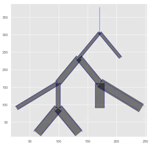
        ax.plot((x-np.sin(theta)*w), y+np.cos(theta)*w, color="blue", linestyle=":")
        ax.plot((x+np.sin(theta)*w), y-np.cos(theta)*w, color="blue", linestyle=":")

经过几次思考实验，我意识到需要计算角度，然后相应地调整垫片:

例如，如果该线完全垂直（在90或-90处），则y坐标不会被移动，但x坐标会被移动。对于角度为0或180的线，则相反。

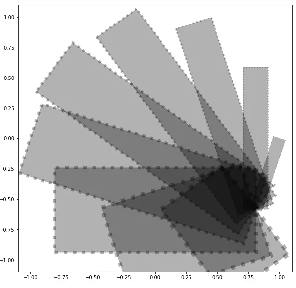
不过，还是有一点偏差。

我怀疑这很相关： matplotlib-如何用数据单位扩展线条宽度？

我认为linewidth不能直接转换为数据空间

或者，如果这些线集合可以转换为矩形对象，则也可以。

- O.rka

---

线宽在您的显示器像素尺寸方面保持不变。一旦调整窗口大小，最初只是“有点偏差”的解决方案将非常“偏离”。个人而言，我不会尝试修复networkx，而是使用数据空间中的坐标绘制对象。 - Paul Brodersen

Answer 1

将一条线用另一条线包围的问题在于，线是在数据坐标系中定义的，而线宽是以物理单位——即点——表示的。这通常是可取的，因为它允许线宽独立于数据范围、缩放级别等，同时确保线的末端始终垂直于线，不受轴比例的影响。

因此，线的轮廓始终处于混合坐标系中，在绘制实际线条之前无法确定最终外观。因此，对于考虑（可能会变化的）坐标的解决方案，需要确定当前状态下的图形轮廓。

一种选择是使用新的艺术家，将现有的LineCollection作为输入，并根据线在像素空间中的当前位置创建新的转换。

以下示例中选择了PatchCollection。我们从一个矩形开始，可以对其进行缩放和旋转，然后将其平移到原始线的位置。

import numpy as np
import matplotlib.pyplot as plt
from matplotlib.collections import LineCollection, PatchCollection
import matplotlib.transforms as mtrans


class OutlineCollection(PatchCollection):
    def __init__(self, linecollection, ax=None, **kwargs):
        self.ax = ax or plt.gca()
        self.lc = linecollection
        assert np.all(np.array(self.lc.get_segments()).shape[1:] == np.array((2,2)))
        rect = plt.Rectangle((-.5, -.5), width=1, height=1)
        super().__init__((rect,), **kwargs)
        self.set_transform(mtrans.IdentityTransform())
        self.set_offsets(np.zeros((len(self.lc.get_segments()),2)))
        self.ax.add_collection(self)

    def draw(self, renderer):
        segs = self.lc.get_segments()
        n = len(segs)
        factor = 72/self.ax.figure.dpi
        lws = self.lc.get_linewidth()
        if len(lws) <= 1:
            lws = lws*np.ones(n)
        transforms = []
        for i, (lw, seg) in enumerate(zip(lws, segs)):
            X = self.lc.get_transform().transform(seg)
            mean = X.mean(axis=0)
            angle = np.arctan2(*np.squeeze(np.diff(X, axis=0))[::-1])
            length = np.sqrt(np.sum(np.diff(X, axis=0)**2))
            trans = mtrans.Affine2D().scale(length,lw/factor).rotate(angle).translate(*mean)
            transforms.append(trans.get_matrix())
        self._transforms = transforms
        super().draw(renderer)

请注意实际的变换只在绘制时计算。这确保了它们考虑了像素空间中的实际位置。

用法可能如下所示：

verts = np.array([[[5,10],[5,5]], [[5,5],[8,2]], [[5,5],[1,4]], [[1,4],[2,0]]])

plt.rcParams["axes.xmargin"] = 0.1
fig, (ax1, ax2) = plt.subplots(ncols=2, sharex=True, sharey=True)

lc1 = LineCollection(verts, color="k", alpha=0.5, linewidth=20)
ax1.add_collection(lc1)

olc1 = OutlineCollection(lc1, ax=ax1, linewidth=2, 
                         linestyle=":", edgecolor="black", facecolor="none")


lc2 = LineCollection(verts, color="k", alpha=0.3, linewidth=(10,20,40,15))
ax2.add_collection(lc2)

olc2 = OutlineCollection(lc2, ax=ax2, linewidth=3, 
                         linestyle="--", edgecolors=["r", "b", "gold", "indigo"], 
                        facecolor="none")

for ax in (ax1,ax2):
    ax.autoscale()
plt.show()

现在的想法是使用来自问题的 linecollection 对象，而不是上面的 lc1 对象。在代码中应该很容易替换。

- ImportanceOfBeingErnest

---

我终于想出如何为此调整我的代码了！谢谢。这是一个巨大的答案。我知道这可能需要一些时间。我不知道它会这么复杂，但你说的很有道理。 - O.rka

你有没有对如何使其适应输出为 FancyArrowPatch 对象的 nx.DiGraph 对象的建议？我曾尝试使用 PatchCollection([FancyArrowPatches from nx.draw_networkx_edges])，但我得到了 AttributeError: 'PatchCollection' object has no attribute 'get_segments'。 - O.rka

你是说你根本没有“LineCollection”吗？还是这是一个新问题？FancyArrowPatches可以是弧形或者其他弯曲的形状，因此需要使用完全不同的策略。 - ImportanceOfBeingErnest

当我将我的真实数据复制成简化形式用于此帖子时，我使用了nx.Graph而不是我的原始nx.OrderedDiGraph。我已经完美地使用了您的方法来处理nx.Graph（再次感谢），但没有意识到nx.OrderedDiGraph返回一个FancyArrowPatches列表。我几乎已经调整好脚本以将其合并https://pastebin.com/raw/jzL92vdW，但在最终图中出现了奇怪的偏移https://i.imgur.com/sQys7Jz.png。 - O.rka

我目前没有可运行的networkx，并且在接下来的一周左右可能无法进一步研究此问题。 - ImportanceOfBeingErnest

最后我在nx.draw_networkx_edges中使用了arrows=False选项，所以现在它可以工作了！虽然不是FancyArrowPatch，但没关系...因为这不是我所尝试做的必要条件。干杯 - O.rka

Answer 2

LineCollection中的对象没有明显的边缘颜色和面颜色。尝试设置线型会影响整个线段的样式。我发现使用一系列补丁来创建所需效果更容易。每个补丁表示图形的一个边缘。可以分别操纵补丁的边缘颜色、线型、线宽和面颜色。关键是构建一个函数，将边缘转换为旋转的矩形补丁。

import matplotlib.path as mpath
import matplotlib.patches as mpatches
import numpy as np
from matplotlib import pyplot as plt
import networkx as nx

G = nx.Graph()
for i in range(10):
    G.add_node(i)
for i in range(9):
    G.add_edge(9, i)

# make a square figure so the rectangles look nice
plt.figure(figsize=(10,10))
plt.xlim(-1.1, 1.1)
plt.ylim(-1.1, 1.1)

def create_patch(startx, starty, stopx, stopy, width, w=.1):
    # Check if lower right corner is specified.
    direction = 1
    if startx > stopx:
        direction = -1

    length = np.sqrt((stopy-starty)**2 + (stopx-startx)**2)
    theta = np.arctan((stopy-starty)/(stopx-startx))
    complement = np.pi/2 - theta

    patch = mpatches.Rectangle(
        (startx+np.cos(complement)*width/2, starty-np.sin(complement)*width/2), 
        direction * length,
        width,
        angle=180/np.pi*theta, 
        facecolor='#000000', 
        linestyle=':', 
        linewidth=width*10,
        edgecolor='k',
        alpha=.3
    )
    return patch

# Create layout before building edge patches
pos = nx.circular_layout(G)

for i, edge in enumerate(G.edges()):
    startx, starty = pos[edge[0]]
    stopx, stopy = pos[edge[1]]
    plt.gca().add_patch(create_patch(startx, starty, stopx, stopy, (i+1)/10))

plt.show()

在你的示例中，你注意到我们可以使用边缘的X和Y位置来找到旋转角度。我们在这里使用同样的技巧。还要注意有时矩形长度的大小为负数。矩形补丁假设x和y输入是矩形左下角。我们运行一个快速检查以确保这是正确的。如果不是，则我们指定了顶部。在这种情况下，我们沿着相同的角度向后绘制矩形。

另一个需要注意的问题：在创建补丁之前运行布局算法非常重要。一旦指定了pos，我们就可以使用边缘查找起始和停止位置。 改进机会：与其在生成每个补丁时绘制它，你可以使用PatchCollection并批量操作补丁。文档声称PatchCollection更快，但它可能不适用于所有用例。由于你表达了希望单独设置每个补丁的属性，所以集合可能不提供你需要的灵活性。

- SNygard

---

这里的主要假设是图表以等比例显示（即y方向上的一个单位与x方向上的一个单位具有相同的长度）。根据问题中的图片，情况并非必然如此。 - ImportanceOfBeingErnest

这是一个很好的观点。我得考虑如何在其他宽高比方面处理它（理想情况下，我们不需要提前知道宽高比...） - SNygard

当我在我的示例中使用时： ZeroDivisionError: theta = np.arctan((stopy-starty)/(stopx-startx)) ZeroDivisionError: 浮点数除以零 - O.rka