使用ggpmisc显示nls模型的方程式

Question

R包ggpmisc可以用来在ggplot2上显示lm模型和poly模型的方程（参见这里）。 我想知道如何使用ggpmisc在ggplot2上显示nls模型方程结果。下面是我的最小工作示例。

library(ggpmisc)
args <- list(formula = y ~ k * e ^ x,
             start = list(k = 1, e = 2))
ggplot(mtcars, aes(wt, mpg)) +
  geom_point() +
  stat_fit_augment(method = "nls",
                   method.args = args)

- MYaseen208

Answer 1

受您提供的帖子启发。使用geom_text在提取参数后添加标签。

nlsFit <-
  nls(formula = mpg ~ k * e ^ wt,
      start = list(k = 1, e = 2),
      data = mtcars)

nlsParams <-
  nlsFit$m$getAllPars()

nlsEqn <-
  substitute(italic(y) == k %.% e ^ italic(x), 
             list(k = format(nlsParams['k'], digits = 4), 
                  e = format(nlsParams['e'], digits = 2)))

nlsTxt <-
  as.character(as.expression(nlsEqn))

ggplot(mtcars, aes(wt, mpg)) +
  geom_point() +
  stat_fit_augment(method = "nls",
                   method.args = args) + 
  geom_text(x = 5, y = 30, label = nlsTxt, parse = TRUE)

- Mir Henglin

---

由于某些原因，值被c()封装。y = c(value) e ^ c(value): nlsTxt [1] "italic(y) == c(k = \"49.66\") %.% c(e = \"0.75\")^italic(x)" - Aliton Oliveira

Answer 2

使用'ggpmisc'包可以通过组合要使用paste()或sprintf()解析的字符字符串来添加方程。在这个回答中，我将使用sprintf()。我使用它所包含的示例回答问题。我在这个回答中没有展示，但这种方法支持分组和面板。缺点是模型需要拟合两次，一次绘制拟合线，一次添加方程。

为了找到由stat_fit_tidy()返回的变量名称，我使用了'gginnards'包中的geom_debug()，尽管名称依赖于模型公式和方法，但它们相当容易预测。除了添加一个图层geom_debug()外，还会将其data输入回显到R控制台上。接下来，一旦我们知道要在标签中使用的变量的名称，我们就可以组装要作为R表达式解析的字符串。

使用 sprintf() 组装标签时，需要将 % 字符转义为 %%，以便原样返回，因此乘号 %*% 变为 %%*%%。在 R 表达式中嵌入字符字符串是可能的，而且在这种情况下很有用，但我们需要将嵌入的引号转义为 \"。

library(tidyverse)
library(ggpmisc)
#> Loading required package: ggpp
#> 
#> Attaching package: 'ggpp'
#> The following object is masked from 'package:ggplot2':
#> 
#>     annotate
library(gginnards)

args <- list(formula = y ~ k * e ^ x,
             start = list(k = 1, e = 2))

# we find the names of computed values
ggplot(mtcars, aes(wt, mpg)) +
  stat_fit_tidy(method = "nls",
                method.args = args,
                geom = "debug")

#> Input 'data' to 'draw_panel()':
#>   npcx npcy k_estimate e_estimate     k_se       e_se   k_stat   e_stat
#> 1   NA   NA   49.65969  0.7455911 3.788755 0.01985924 13.10713 37.54378
#>      k_p.value    e_p.value       x      y fm.class fm.method  fm.formula
#> 1 5.963165e-14 8.861929e-27 1.70855 32.725      nls       nls y ~ k * e^x
#>   fm.formula.chr PANEL group
#> 1    y ~ k * e^x     1    -1

# plot with formula
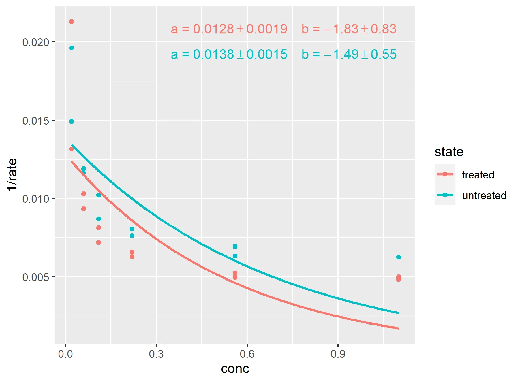
ggplot(mtcars, aes(wt, mpg)) +
  geom_point() +
  stat_fit_augment(method = "nls",
                   method.args = args) +
  stat_fit_tidy(method = "nls",
                method.args = args,
                label.x = "right",
                label.y = "top",
                aes(label = sprintf("\"mpg\"~`=`~%.3g %%*%% %.3g^{\"wt\"}",
                                    after_stat(k_estimate),
                                    after_stat(e_estimate))),
                parse = TRUE )

^{创建于2022年9月2日，使用 reprex v2.0.2}

- Pedro J. Aphalo

---

check_subclass() 函数出错： ！无法找到名为“debug”的 geom。 - Aliton Oliveira

你运行了 library(gginnards) 吗？ - Pedro J. Aphalo

Answer 3

这里我展示了使用ggpmisc的nls与分组来添加到绘图中，使用当前的CRAN ggpmisc（v 0.3.8）。这是vignette的变化/修改，其中'stat_fit_tidy（）'使用michaelis-menten拟合，可以在here找到。 输出看起来像这样：

library(tidyverse)
library(tidymodels)
library(ggpmisc)

my_exp_formula <-  y ~ a * exp(b*x-0)
# if x has large values (i.e. >700), subtract the minimum
# see https://stackoverflow.com/a/41108403/4927395

#example with nls, shows the data returned
o <- nls(1/rate ~ a * exp(b*conc-0), data = Puromycin, start = list(a = 1, b = 2))
o
tidy(o)

ggplot(Puromycin, aes(conc, 1/rate, colour = state)) +
  geom_point() +
  geom_smooth(method = "nls", 
              formula = my_exp_formula,
              se = FALSE) +
  stat_fit_tidy(method = "nls", 
                method.args = list(formula = my_exp_formula),
                label.x = "right",
                label.y = "top",
                aes(label = paste("a~`=`~", signif(stat(a_estimate), digits = 3),
                                  "%+-%", signif(stat(a_se), digits = 2),
                                  "~~~~b~`=`~", signif(stat(b_estimate), digits = 3),
                                  "%+-%", signif(stat(b_se), digits = 2),
                                  sep = "")),
                parse = TRUE)
ggsave("exp plot.png")

- Mark Neal