使用分类变量拟合nls模型。

Question

我希望拟合一个线性-平台（nls）模型，描述身高随年龄变化的关系，并测试模型参数在不同地区是否存在显著差异。

这是目前的进展：

# Create data
df1 <- cbind.data.frame (height = c (0.5, 0.6, 0.9, 1.3, 1.5, 1.6, 1.6,
                                     0.6, 0.6, 0.8, 1.3, 1.5, 1.6, 1.5,
                                     0.6, 0.8, 1.0, 1.4, 1.6, 1.6, 1.6,
                                     0.5, 0.8, 1.0, 1.3, 1.6, 1.7, 1.6),
                         age = c (0.5, 0.9, 3.0, 7.3, 12.2, 15.5, 20.0,
                                  0.4, 0.8, 2.3, 8.5, 11.5, 14.8, 21.3,
                                  0.5, 1.0, 5.1, 11.1, 12.3, 16.0, 19.8,
                                  0.5, 1.1, 5.5, 10.2, 12.2, 15.4, 20.5),
                         region = as.factor (c (rep ("A", 7),
                                                rep ("B", 7),
                                                rep ("C", 7),
                                                rep ("D", 7))))

> head (df1)
  height  age region
1    0.5  0.5      A
2    0.6  0.9      A
3    0.9  3.0      A
4    1.3  7.3      A
5    1.5 12.2      A
6    1.6 15.5      A

# Create linear-plateau function
lp <- function(x, a, b, c){
  ifelse (x < c, a + b * x, a + b * c)
  } # Where 'a' is the intercept, 'b' the slope and 'c' the breakpoint

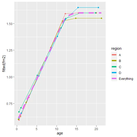
# Fit the model ignoring region
m1 <- nls (height ~ lp (x = age, a, b, c),
           data = df1,
           start = list (a = 0.5, b = 0.1, c = 13))

> summary (m1)

Formula: height ~ lp(x = age, a, b, c)

Parameters:
   Estimate Std. Error t value Pr(>|t|)    
a  0.582632   0.025355   22.98   <2e-16 ***
b  0.079957   0.003569   22.40   <2e-16 ***
c 12.723995   0.511067   24.90   <2e-16 ***
---
Signif. codes:  0 ‘***’ 0.001 ‘**’ 0.01 ‘*’ 0.05 ‘.’ 0.1 ‘ ’ 1

Residual standard error: 0.07468 on 25 degrees of freedom

Number of iterations to convergence: 2 
Achieved convergence tolerance: 5.255e-09

我想要用相同的模型来考虑“region”，并测试“a”、“b”和“c”的估计值在不同地区是否不同。

我认为这篇帖子可能有用，但我不知道如何将其应用于此数据/函数。

以下是数据的外观：

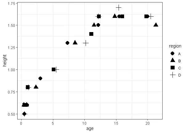
非使用nls的解决方案也受欢迎。

- Enrique Otero

Answer 1

使用相同的参数为每个区域拟合模型，得到fm1，然后使用不同的参数得到fm2，并使用anova测试它们之间的差异。

我们使用plinear算法来拟合fm1，因为它消除了线性参数的起始值需求。在这种情况下，RHS应该是一个矩阵，其第一列乘以截距，第二列乘以斜率。这两个线性参数将被命名为.lin1和.lin2。我们重复fm1拟合中的系数四次作为fm2拟合的起始值。

fm1 <- nls(height ~ cbind(1, pmin(age, c)), df1, start = list(c = mean(df1$age)),
  algorithm = "plinear")
co <- as.list(coef(fm1))

fm2 <- nls(height ~ a[region] + b[region] * pmin(age, c[region]), df1, 
  start = list(a = rep(co$.lin1, 4), b = rep(co$.lin2, 4), c = rep(co$c, 4)))

anova(fm1, fm2)

提供：

Analysis of Variance Table

Model 1: height ~ cbind(1, pmin(age, c))
Model 2: height ~ a[region] + b[region] * pmin(age, c[region])
  Res.Df Res.Sum Sq Df   Sum Sq F value Pr(>F)
1     25    0.13944                           
2     16    0.11895  9 0.020483  0.3061 0.9617

因此，我们无法拒绝参数在不同地区相同的假设。

如果我们想测试不同的c值但具有共同的截距和斜率，我们可以使用

fm3 <- nls(height ~ cbind(1, pmin(age, c[region])), df1, 
   start = list(c = rep(co$c, 4)), algorithm = "plinear")

anova(fm1, fm3)

虽然我们无法用肉眼判断c值在不同区域间是否相同，但从下面的可视化图表中可以看出，平稳值的截止年龄似乎有所不同，因此我们可能想要使用fm3，尽管它与fm1没有显著差异。在这里，我们可能希望根据与应用程序相关的其他因素来指导选择，而不仅仅是拟合程度。

图形

以下是fm2的各个拟合结果以及fm1的整体拟合结果。

library(ggplot2)

df1$Everything <- "Everything"
ggplot(df1, aes(age, fitted(fm2), col = region)) +
  geom_line() +
  geom_point() +
  geom_line(aes(age, fitted(fm1), col = Everything), lty = 2, lwd = 2)

- G. Grothendieck