使用gtable/grob在ggplot中自定义标签元素位置

Question

使用gtable/grob在ggplot中自定义标签元素位置

4

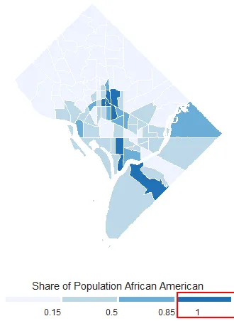
我正在使用R中的ggplot创建DC地图。我尝试自定义图例栏和标签。我可以移动图例键，但无法移动标签，使用gtable_filter。我希望将最后一个标签“1”移近其图例栏，就像其他标签一样。感谢任何帮助。地图图片我正在使用以下R代码：

Data set looks like below

    head(d1930)

R Output:



     Simple feature collection with 6 features and 355 fields
            geometry type:  MULTIPOLYGON
            dimension:      XY
            bbox:           xmin: -77.0823 ymin: 38.89061 xmax: -77.0446 ymax: 38.94211
            epsg (SRID):    4326
            proj4string:    +proj=longlat +datum=WGS84 +no_defs
              fipsstate fipscounty  tract NHGISST NHGISCTY      GISJOIN    GISJOIN2 SHAPE_AREA SHAPE_LEN  X  GISJOIN.x.1 year cenv1_1 cenv8_1
            1        11        001 000001     110     0010 G11000100001 11000100001    1953567  8965.853  1 G11001000001 1930    7889    5885
            2        11        001 000002     110     0010 G11000100002 11000100002    1345844  5668.739 10 G11001000002 1930    6250    5164




       # # borrowed map theme and code from here
        # # https://timogrossenbacher.ch/2016/12/beautiful-thematic-maps-with-ggplot2-only/


            theme_map <- function(...) {
              theme_minimal() +
                theme(
                  text = element_text(family = "Ubuntu Regular", color = "#22211d"),
                  axis.line = element_blank(),
                  axis.text.x = element_blank(),
                  axis.text.y = element_blank(),
                  axis.ticks = element_blank(),
                  axis.title.x = element_blank(),
                  axis.title.y = element_blank(),
                  # panel.grid.minor = element_line(color = "#ebebe5", size = 0.2),
                  panel.grid.major = element_line(color = "white", size = 0.2),
                  panel.grid.minor = element_blank(),
                  plot.background = element_rect(fill = "white", color = NA),
                  panel.background = element_rect(fill = "white", color = NA),
                  legend.background = element_rect(fill = "white", color = NA),
                  panel.border = element_blank(),
                  ...
                )
            }


    # create the color vector

        my.cols <- brewer.pal(4, "Blues")

    # compute labels

        labels <- c()

    # put manual breaks as desired

        brks <- c(0,0.15,0.5,0.85,1)

    # round the labels (actually, only the extremes)

        for(idx in 1:length(brks)){
          labels <- c(labels,round(brks[idx + 1], 2))
        }

    # put labels into label vector

        labels <- labels[1:length(labels)-1]

    # define a new variable on the data set just as above

        d1930$brks <- cut(d1930$pAA, 
                          breaks = brks, 
                          include.lowest = TRUE, 
                          labels = labels)

    # define breaks scale and labels scales

        brks_scale <- levels(d1930$brks)
        labels_scale <- rev(brks_scale)

    # draw the plot with legend at the bottom

        p <- ggplot(d1930) + 
          geom_sf(aes(fill=brks),colour = "white")+
          coord_sf() +
          theme_map() +
          theme(legend.position = "bottom",legend.background = element_rect(color = NA)) 

    # provide manual scale and colors to the graph



    tester <- p +
          # now we have to use a manual scale, 
          # because only ever one number should be shown per label
          scale_fill_manual(
            # in manual scales, one has to define colors, well, we have done it earlier
            values = my.cols,
            breaks = rev(brks_scale),
            name = "Share of Population African American",
            drop = FALSE,
            labels = labels_scale,
            guide = guide_legend(
              direction = "horizontal",
              keyheight = unit(2.5, units = "mm"),
              keywidth = unit(85 / length(labels), units = "mm"),                      title.position = 'top',
              # shift the labels around, the should be placed 
              # exactly at the right end of each legend key
              title.hjust = 0.5,
              label.hjust = 1,                         ### change here 
              nrow = 1,
              byrow = T,
              # also the guide needs to be reversed
              reverse = T,
              label.position = "bottom"
            )
          )

        tester

        library(grid)
        library(gtable)

        extendLegendWithExtremes <- function(p){
          p_grob <- ggplotGrob(p)
          legend <- gtable_filter(p_grob, "guide-box")
          legend_grobs <- legend$grobs[[1]]$grobs[[1]]
          print(legend_grobs)
          # grab the first key of legend
          legend_first_key <- gtable_filter(legend_grobs, "key-3-1-1")
          legend_first_key$widths <- unit(2, units = "cm")
          # modify its width and x properties to make it longer
          legend_first_key$grobs[[1]]$width <- unit(1, units = "cm")
          legend_first_key$grobs[[1]]$x <- unit(1.6, units = "cm")              

          # last key of legend
          legend_last_key <- gtable_filter(legend_grobs, "key-3-4-1")
          legend_last_key$widths <- unit(2, units = "cm")

          # analogous
          legend_last_key$grobs[[1]]$width <- unit(1, units = "cm")
          legend_last_key$grobs[[1]]$x <- unit(0.5, units = "cm")

          # grab the last label so we can also shift its position 
    # below code is where i am stuck as this is not shifting the label
          legend_last_label <- gtable_filter(legend_grobs, "label-5-4")
          legend_last_label$widths <- unit(20, units = "cm")
          legend_last_label$grobs[[1]]$x <- unit(-10.1, units = "cm")
          legend_last_label$grobs[[1]]$width <- unit(10, units = "cm")

    # Insert new color legend back into the combined legend
          legend_grobs$grobs[legend_grobs$layout$name == "key-3-1-1"][[1]] <- 
            legend_first_key$grobs[[1]]
          legend_grobs$grobs[legend_grobs$layout$name == "key-3-4-1"][[1]] <- 
            legend_last_key$grobs[[1]]
          legend_grobs$grobs[legend_grobs$layout$name == "label-5-4"][[1]] <- 
            legend_last_label$grobs[[1]]  


          legend$grobs[[1]]$grobs[1][[1]] <- legend_grobs
          p_grob$grobs[p_grob$layout$name == "guide-box"][[1]] <- legend

          # the plot is now drawn using this grid function
          grid.newpage()
          grid.draw(p_grob)
          print(legend_grobs)
          # save the plot
          ggsave(paste0("~/Desktop/RA/",dateo,"_dc_1930.jpg"),
                              plot = p_grob, dpi = 300, width = 11, height = 8.5, units = c("in"))
        }

        extendLegendWithExtremes(tester)

- Deepak

2

请使用 dput() 函数分享您的数据样本（不要使用 str、head 或图片/截图），以便他人提供帮助。更多信息请参见 https://dev59.com/eG025IYBdhLWcg3whGSx?rq=1 - Tung

谢谢@Tung，我已经将数据上传到我的github存储库中，同时提供了rds和csv格式。以下是rds格式的数据链接：https://github.com/iamdeepaka/Data-Mining-using-R/blob/master/d1930.rds - Deepak

1个回答

网页内容由stack overflow 提供, 点击上面的

可以查看英文原文，
原文链接

- Valentin_Ștefan · Accepted Answer

你是否没有准确获取最后一个标签的坐标？例如，legend_last_label$grobs [[1]] $ x 为NULL，而应该返回1npc。以下是一种获取它的方法：

legend_last_label$grobs[[1]][["children"]][[1]][["children"]][[1]][["x"]]
#> [1] 1npc
# Overwrite it as you wish:
legend_last_label$grobs[[1]][["children"]][[1]][["children"]][[1]][["x"]] <- unit(-1, units = "cm")

也许更安全的做法是使用每个图形对象的来“捕捉”它们，然后使用函数进行编辑。下面是一个应用在你的绘图上的示例：

g <- grid.force(ggplotGrob(tester)) # get all grobs and their components
grid.ls(g) # list the names of all grobs

传说的位置在底部某处，标识为“guide-box.etc”。

#>   guide-box.11-5-11-5
#>     legend.box.background.2-4-4-2
#>     guides.3-3-3-3
#>       background.1-7-7-1
#>       title.2-6-2-2
#>         guide.title.titleGrob.123
#>           GRID.text.121
#>       key-3-1-bg.4-2-4-2
#>       key-3-1-1.4-2-4-2
#>       key-3-2-bg.4-3-4-3
#>       key-3-2-1.4-3-4-3
#>       key-3-3-bg.4-4-4-4
#>       key-3-3-1.4-4-4-4
#>       key-3-4-bg.4-5-4-5
#>       key-3-4-1.4-5-4-5
#>       label-5-1.6-2-6-2
#>         guide.label.titleGrob.126
#>           GRID.text.124
#>       label-5-2.6-3-6-3
#>         guide.label.titleGrob.129
#>           GRID.text.127
#>       label-5-3.6-4-6-4
#>         guide.label.titleGrob.132
#>           GRID.text.130
#>       label-5-4.6-5-6-5
#>         guide.label.titleGrob.135
#>           GRID.text.133

你的最后一个标签被称为：

#>       label-5-4.6-5-6-5
#>         guide.label.titleGrob.135
#>           GRID.text.133

现在我们需要为每个grob构建gPath。也许有更简单的方法，但这是一种方法：

# delete "layout::" from raw gPath & add grob name at the end
gpaths <- paste(gsub(pattern = "layout::", 
                       replacement = "", 
                       x = grid.ls(g, print = FALSE)$gPath), 
                  grid.ls(g, print = FALSE)$name, 
                  sep = "::")

您的标签文本路径为：

gpaths[grepl("guide-box.*label-5-4.*GRID\\.text.*", gpaths)]
#> [1] "guide-box.11-5-11-5::guides.3-3-3-3::label-5-4.6-5-6-5::guide.label.titleGrob.135::GRID.text.133"

所以，有了路径之后，我们可以编辑grob，即将标签向左移动：

g <- editGrob(grob = g, 
              gPath = gpaths[grepl("guide-box.*label-5-4.*GRID.text.*", gpaths)], 
              x = unit(-1, "cm"))
plot(g)

此外，您可以编辑按键的宽度和位置。以下是编辑最右边按键的方法：

g <- editGrob(grob = g, 
              gPath = gpaths[grepl("guide-box.*key-3-4-1.*", gpaths)], 
              x = unit(0.5, "cm"),
              width = unit(1, "cm"))
plot(g)

此外，我认为你应该将labels <- labels[1:length(labels)-1]替换为labels <- labels[-length(labels)];否则，在构建d1930$brks时，将会从cut函数中得到一个错误。