我想使用ggplot2包将两个图并排放置,即相当于执行par(mfrow=c(1,2))命令。
例如,我希望以下两个图像能够并排显示,并具有相同的比例。
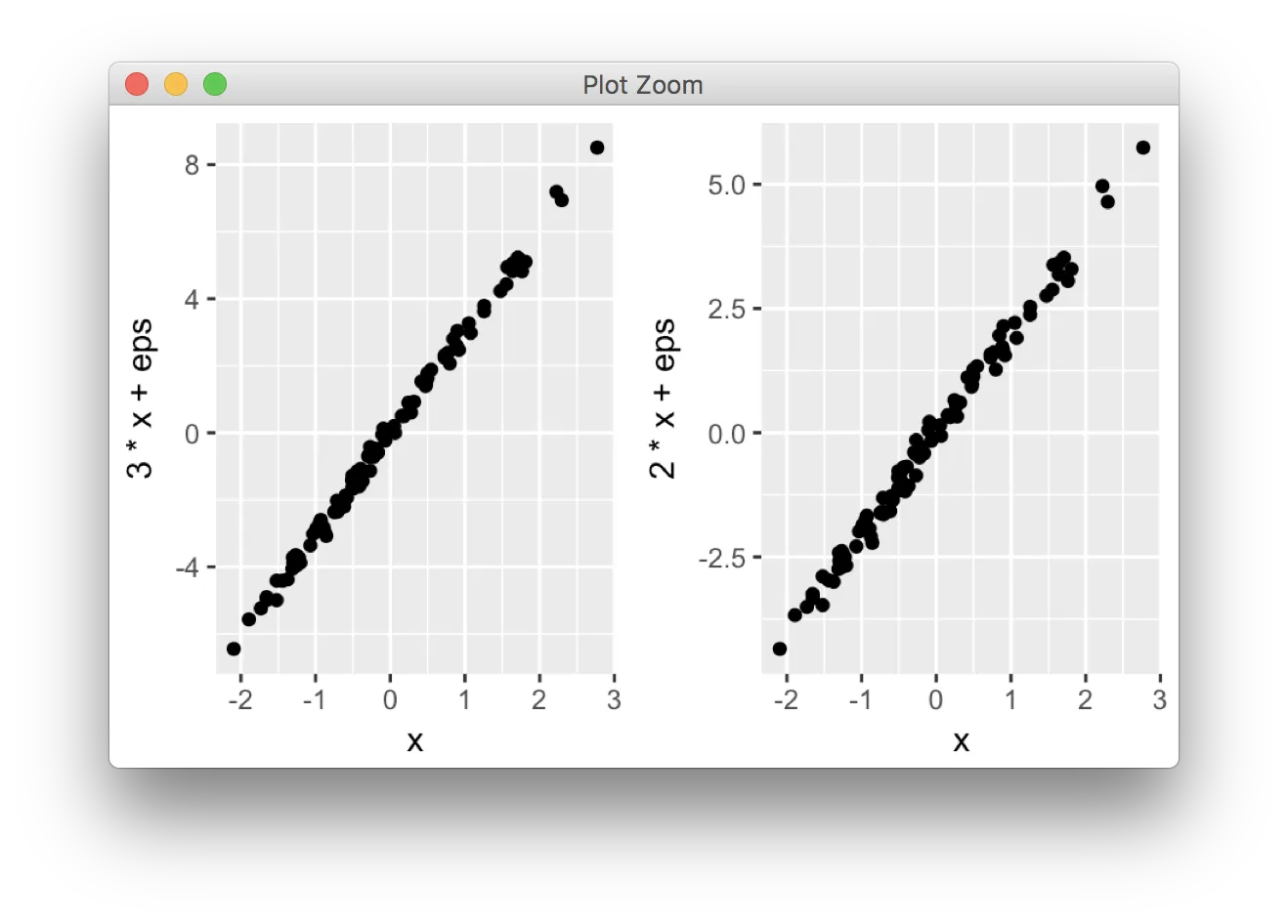
x <- rnorm(100)
eps <- rnorm(100,0,.2)
qplot(x,3*x+eps)
qplot(x,2*x+eps)
我需要把它们放在同一个数据框中吗?
qplot(displ, hwy, data=mpg, facets = . ~ year) + geom_smooth()
我想使用ggplot2包将两个图并排放置,即相当于执行par(mfrow=c(1,2))命令。
例如,我希望以下两个图像能够并排显示,并具有相同的比例。
x <- rnorm(100)
eps <- rnorm(100,0,.2)
qplot(x,3*x+eps)
qplot(x,2*x+eps)
我需要把它们放在同一个数据框中吗?
qplot(displ, hwy, data=mpg, facets = . ~ year) + geom_smooth()
gridExtra包中的函数grid.arrange()可以结合多个图形展示;通过这个函数,你可以将两个图像并排显示。
require(gridExtra)
plot1 <- qplot(1)
plot2 <- qplot(1)
grid.arrange(plot1, plot2, ncol=2)
当两个图表不基于相同的数据时,这很有用,例如如果您想绘制不同的变量而不使用reshape()。
这将作为副作用来绘制输出。要将副作用打印到文件中,请指定设备驱动程序(例如pdf,png等),例如:
pdf("foo.pdf")
grid.arrange(plot1, plot2)
dev.off()
或者,使用arrangeGrob()与ggsave()结合使用,
ggsave("foo.pdf", arrangeGrob(plot1, plot2))
这相当于使用par(mfrow = c(1,2))制作两个不同的图。这不仅节省了排列数据的时间,而且在您想要两个不同的图时是必要的。
对于为不同组制作类似的图形,面板非常有用。如下所述,在许多回答中都指出了这一点,但我想通过等同于上述图形的示例来强调这种方法。
mydata <- data.frame(myGroup = c('a', 'b'), myX = c(1,1))

qplot(data = mydata,
    x = myX,
    facets = ~myGroup)

ggplot(data = mydata) +
    geom_bar(aes(myX)) +
    facet_wrap(~myGroup)
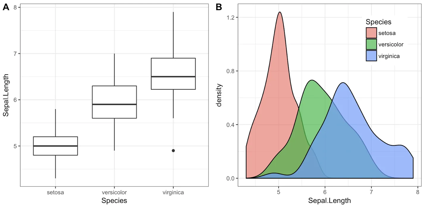
值得一提的是,cowplot包中的plot_grid函数可以作为grid.arrange的替代品。请参考@claus-wilke在下面的回答以及此vignette获取等效方法;但是该函数允许基于此vignette对图形位置和大小进行更细致的控制。
?grid.arrange 让我想到这个函数现在被称为 arrangeGrob。我通过 a <- arrangeGrob(p1, p2) 然后 print(a) 实现了我想做的事情。 - blakeoftgrid.arrange仍然是一个有效的、未被弃用的函数。你尝试使用这个函数了吗?如果没有,那么发生了什么,如果不是你期望的结果呢? - David LeBauergrid.arrange 的解决方案的一个缺点是,它们使得在图中用字母(A、B 等)标记绘图变得困难,因为大多数期刊都要求这样做。< /p >
< p >我编写了 cowplot 包来解决这个问题(以及其他一些问题),具体来说是使用函数 plot_grid():< /p >
library(cowplot)

iris1 <- ggplot(iris, aes(x = Species, y = Sepal.Length)) +
  geom_boxplot() + theme_bw()

iris2 <- ggplot(iris, aes(x = Sepal.Length, fill = Species)) +
  geom_density(alpha = 0.7) + theme_bw() +
  theme(legend.position = c(0.8, 0.8))

plot_grid(iris1, iris2, labels = "AUTO")
plot_grid() 返回的对象是另一个 ggplot2 对象,您可以像往常一样使用 ggsave() 将其保存:p <- plot_grid(iris1, iris2, labels = "AUTO")
ggsave("plot.pdf", p)
另外,您可以使用cowplot函数save_plot(),它是对ggsave()的轻量级包装,使得获取合并图的正确尺寸变得更加容易,例如:
p <- plot_grid(iris1, iris2, labels = "AUTO")
save_plot("plot.pdf", p, ncol = 2)
ncol = 2参数告诉save_plot()有两个并排的图,save_plot()使保存的图像宽度加倍。)
有关如何在网格中排列图形的更深入描述,请参见this vignette. 还有一篇解释如何制作具有shared legend.的图例的vignette。
一个常见的困惑点是cowplot包更改了默认的ggplot2主题。该包的行为方式是这样的,因为它最初是为内部实验室使用而编写的,我们从不使用默认主题。如果这会引起问题,您可以使用以下三种方法之一来解决它们:
1. 为每个图手动设置主题。我认为始终为每个图指定特定的主题是一个好习惯,就像我在上面的示例中使用+ theme_bw()一样。如果您指定了特定的主题,则默认主题无关紧要。
2. 将默认主题恢复为ggplot2默认主题。 您可以使用一行代码完成此操作:
theme_set(theme_gray())
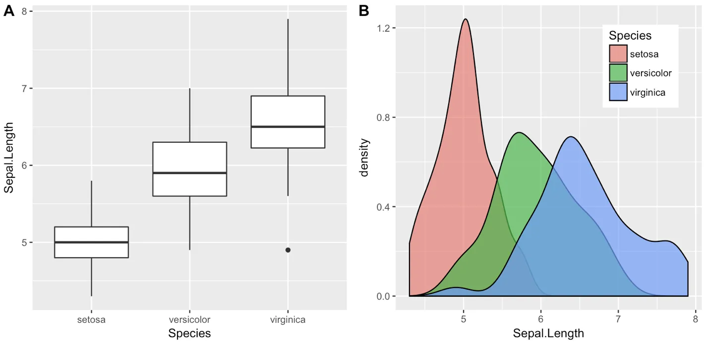
3. 不需要加载cowplot包就能使用其函数。您也可以不调用library(cowplot)或require(cowplot),而是通过在函数前加上cowplot::来调用cowplot函数。例如,使用ggplot2默认主题的上述示例将变为:
## Commented out, we don't call this
# library(cowplot)

iris1 <- ggplot(iris, aes(x = Species, y = Sepal.Length)) +
  geom_boxplot()

iris2 <- ggplot(iris, aes(x = Sepal.Length, fill = Species)) +
  geom_density(alpha = 0.7) +
  theme(legend.position = c(0.8, 0.8))

cowplot::plot_grid(iris1, iris2, labels = "AUTO")
更新:
plot_grid()指定面板大小?我刚试过使用它,但它压缩了我的图像。也许在使用plot_grid()之前需要指定ggplot图像的大小? - David Irelandmultiplot函数。multiplot(plot1, plot2, cols=2)
multiplot <- function(..., plotlist=NULL, cols) {
    require(grid)

    # Make a list from the ... arguments and plotlist
    plots <- c(list(...), plotlist)

    numPlots = length(plots)

    # Make the panel
    plotCols = cols                          # Number of columns of plots
    plotRows = ceiling(numPlots/plotCols) # Number of rows needed, calculated from # of cols

    # Set up the page
    grid.newpage()
    pushViewport(viewport(layout = grid.layout(plotRows, plotCols)))
    vplayout <- function(x, y)
        viewport(layout.pos.row = x, layout.pos.col = y)

    # Make each plot, in the correct location
    for (i in 1:numPlots) {
        curRow = ceiling(i/plotCols)
        curCol = (i-1) %% plotCols + 1
        print(plots[[i]], vp = vplayout(curRow, curCol ))
    }

}
是的,我认为您需要适当地安排数据。一种方法是这样的:
X <- data.frame(x=rep(x,2),
                y=c(3*x+eps, 2*x+eps),
                case=rep(c("first","second"), each=100))

qplot(x, y, data=X, facets = . ~ case) + geom_smooth()
我相信plyr或reshape中有更好的技巧 - 我还没有完全掌握Hadley开发的所有这些强大的包。
使用reshape包,您可以像这样操作。
library(ggplot2)
wide <- data.frame(x = rnorm(100), eps = rnorm(100, 0, .2))
wide$first <- with(wide, 3 * x + eps)
wide$second <- with(wide, 2 * x + eps)
long <- melt(wide, id.vars = c("x", "eps"))
ggplot(long, aes(x = x, y = value)) + geom_smooth() + geom_point() + facet_grid(.~ variable)
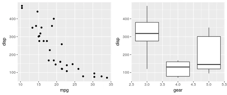
library(ggplot2)
theme_set(theme_bw())

q1 <- ggplot(mtcars) + geom_point(aes(mpg, disp))
q2 <- ggplot(mtcars) + geom_boxplot(aes(gear, disp, group = gear))
q3 <- ggplot(mtcars) + geom_smooth(aes(disp, qsec))
q4 <- ggplot(mtcars) + geom_bar(aes(carb))

library(magrittr)
library(multipanelfigure)
figure1 <- multi_panel_figure(columns = 2, rows = 2, panel_label_type = "none")
# show the layout
figure1

figure1 %<>%
  fill_panel(q1, column = 1, row = 1) %<>%
  fill_panel(q2, column = 2, row = 1) %<>%
  fill_panel(q3, column = 1, row = 2) %<>%
  fill_panel(q4, column = 2, row = 2)
figure1

# complex layout
figure2 <- multi_panel_figure(columns = 3, rows = 3, panel_label_type = "upper-roman")
figure2

figure2 %<>%
  fill_panel(q1, column = 1:2, row = 1) %<>%
  fill_panel(q2, column = 3, row = 1) %<>%
  fill_panel(q3, column = 1, row = 2) %<>%
  fill_panel(q4, column = 2:3, row = 2:3)
figure2

由reprex包(v0.2.0.9000)于2018-07-06创建。
ggplot2基于网格图形(grid graphics)开发,该系统为在页面上布置绘图提供了一个不同的系统。与par(mfrow...)命令不同,网格对象(称为grobs)不一定立即绘制,而可以作为常规R对象进行存储和操作,然后再转换为图形输出。这比基本图形的现在就绘制模型具有更大的灵活性,但策略必须有所不同。
我编写了grid.arrange()以提供一个简单的界面,尽可能接近par(mfrow)。在最简单的形式中,代码如下:
library(ggplot2)
x <- rnorm(100)
eps <- rnorm(100,0,.2)
p1 <- qplot(x,3*x+eps)
p2 <- qplot(x,2*x+eps)

library(gridExtra)
grid.arrange(p1, p2, ncol = 2)
更多选项详见这个文档。
一个普遍的抱怨是绘图不一定对齐,比如当它们具有不同大小的轴标签时,但这是设计意图: grid.arrange不会特别处理ggplot2对象,并将其与其他grobs(例如lattice plots)视为相等。它只是在矩形布局中放置grobs。
对于ggplot2对象的特殊情况,我写了另一个函数ggarrange,具有类似的接口,它尝试对齐图形面板(包括分面图),并在用户定义的条件下尝试保持纵横比。
library(egg)
ggarrange(p1, p2, ncol = 2)
这两个函数与ggsave()兼容。如需了解不同选项的概述和一些历史背景,此文档提供了更多信息。
更新:这个答案非常老了。现在推荐使用gridExtra::grid.arrange()来处理。
我把它留在这里,以防有用。
Stephen Turner 在Getting Genetics Done博客上发布了arrange()函数(有关应用说明,请参见帖子)
vp.layout <- function(x, y) viewport(layout.pos.row=x, layout.pos.col=y)
arrange <- function(..., nrow=NULL, ncol=NULL, as.table=FALSE) {
 dots <- list(...)
 n <- length(dots)
 if(is.null(nrow) & is.null(ncol)) { nrow = floor(n/2) ; ncol = ceiling(n/nrow)}
 if(is.null(nrow)) { nrow = ceiling(n/ncol)}
 if(is.null(ncol)) { ncol = ceiling(n/nrow)}
        ## NOTE see n2mfrow in grDevices for possible alternative
grid.newpage()
pushViewport(viewport(layout=grid.layout(nrow,ncol) ) )
 ii.p <- 1
 for(ii.row in seq(1, nrow)){
 ii.table.row <- ii.row
 if(as.table) {ii.table.row <- nrow - ii.table.row + 1}
  for(ii.col in seq(1, ncol)){
   ii.table <- ii.p
   if(ii.p > n) break
   print(dots[[ii.table]], vp=vp.layout(ii.table.row, ii.col))
   ii.p <- ii.p + 1
  }
 }
}
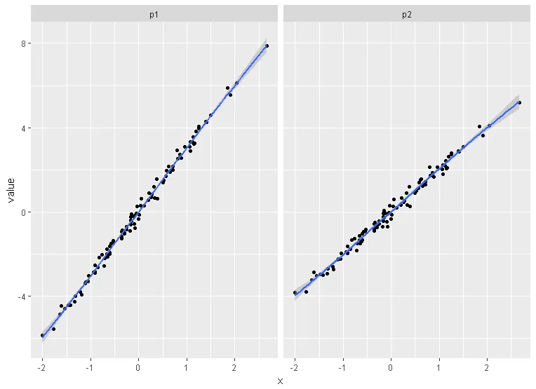
grid.arrange 的一个非常过时的版本(如果我当时没有在邮件列表上发布它,就好了 -- 在线资源无法更新),如果你问我,打包的版本是更好的选择。 - baptiste使用tidyverse:
x <- rnorm(100)
eps <- rnorm(100,0,.2)
df <- data.frame(x, eps) %>%
  mutate(p1 = 3*x+eps, p2 = 2*x+eps) %>%
  tidyr::gather("plot", "value", 3:4) %>%
  ggplot(aes(x = x , y = value)) +
    geom_point() +
    geom_smooth() +
    facet_wrap(~plot, ncol =2)

df