使用Python计算矢量场的散度

Question

有没有可以用于计算矢量场发散的函数？（在 matlab 中）我希望它存在于 numpy/scipy 中，但我无法通过谷歌找到它。

我需要计算 div[A * grad(F)]，其中

F = np.array([[1,2,3,4],[5,6,7,8]]) # (2D numpy ndarray)

A = np.array([[1,2,3,4],[1,2,3,4]]) # (2D numpy ndarray)

所以 grad(F) 是一组2D ndarray 的列表

我知道我可以像this这样计算散度，但不想重复造轮子。（我也希望有更优化的方法）有人有建议吗？

- nyvltak

---

你需要什么顺序的准确性？你的数组是等间距的吗？ - mgilson

http://blog.sun.tc/2010/10/jensenshannon-divergence-in-numpy.html - Dmitry Zagorulkin

@mgilson 是的，数组是等间隔的。我需要双精度。 - nyvltak

@ZagorulkinDmitry，Jensen-Shannon散度是完全不同的东西。 - nyvltak

正确的做法在这里：https://stackoverflow.com/questions/67970477/compute-divergence-with-python/67971515#67971515 - user7086216

Answer 1

给大家一个提示：

上面的函数并不能计算矢量场的散度。它们是对标量场A的导数求和：

结果 = dA / dx + dA / dy

与矢量场不同（以三维为例）：

结果 = sum dAi / dxi = dAx / dx + dAy / dy + dAz / dz

向下投票！这在数学上是错误的。

干杯！

- Polly

---

有点奇怪，这个放在页面底部。其它答案在数学上真的是错误的。 - Daniel

这可能在数学上是正确的，但只是回答问题的第一步。当前的文本并没有回答这个问题。下面有更新的答案实际上回答了手头的问题。 - vidstige

这个答案可以通过告诉我谷歌搜索的问题的答案，以及告诉我其他答案不是我想要的来进行改进。 - Dast

这是正确的做法：https://stackoverflow.com/questions/67970477/compute-divergence-with-python/67971515#67971515 - user7086216

什么？？？上面链接的Matlab函数确实计算了矢量场的散度。你在这里指的是什么？这根本没有任何意义。 - Atcold

Answer 2

import numpy as np

def divergence(field):
    "return the divergence of a n-D field"
    return np.sum(np.gradient(field),axis=0)

- user2818943

---

“field” 是一个标量场。这不会计算出一个向量场的散度。 - Atcold

Answer 3

基于Juh_的答案，但根据矢量场公式的正确散度进行了修改

def divergence(f):
    """
    Computes the divergence of the vector field f, corresponding to dFx/dx + dFy/dy + ...
    :param f: List of ndarrays, where every item of the list is one dimension of the vector field
    :return: Single ndarray of the same shape as each of the items in f, which corresponds to a scalar field
    """
    num_dims = len(f)
    return np.ufunc.reduce(np.add, [np.gradient(f[i], axis=i) for i in range(num_dims)])

Matlab的文档使用了这个确切的公式（向下滚动到矢量场的发散）

- Daniel

Answer 4

@user2818943的答案很好，但可以稍加优化：

def divergence(F):
    """ compute the divergence of n-D scalar field `F` """
    return reduce(np.add,np.gradient(F))

---

Timeit：

F = np.random.rand(100,100)
timeit reduce(np.add,np.gradient(F))
# 1000 loops, best of 3: 318 us per loop

timeit np.sum(np.gradient(F),axis=0)
# 100 loops, best of 3: 2.27 ms per loop

大约快了7倍： sum 隐式地从梯度场列表中构建一个三维数组，这些列表是由np.gradient返回的。使用reduce可以避免这种情况。

---

在您的问题中，div[A * grad(F)]是什么意思？

1. 关于A * grad(F)： A是一个二维数组，grad(f)是一个2d数组列表。因此，我认为它的含义是将每个梯度场与A相乘。
2. 关于在（由A缩放的）梯度场上应用散度不清楚。根据定义，div(F) = d(F)/dx + d(F)/dy + ...。我猜这只是一种表述错误。

对于1，将元素Bi的加和乘以相同的因子A可以因式分解:

Sum(A*Bi) = A*Sum(Bi)

因此，您可以使用以下方法获得加权梯度：A*divergence(F)。

如果A是一个因子列表，每个维度对应一个因子，则解决方案如下：

def weighted_divergence(W,F):
    """
    Return the divergence of n-D array `F` with gradient weighted by `W`

    ̀`W` is a list of factors for each dimension of F: the gradient of `F` over
    the `i`th dimension is multiplied by `W[i]`. Each `W[i]` can be a scalar
    or an array with same (or broadcastable) shape as `F`.
    """
    wGrad = return map(np.multiply, W, np.gradient(F))
    return reduce(np.add,wGrad)

result = weighted_divergence(A,F)

- Juh_

---

矢量场 F 的散度不是等于 d(Fx)/dx + d(Fy)/dy + ... 吗？ 正确的公式应该更像是 np.ufunc.reduce(np.add, [np.gradient(F[i], axis=i) for i in range(len(F))])。 - Daniel

这完全取决于F中的数据类型。问题不太清楚。我有图像处理的经验，因此我认为F是一个n维图像，因此梯度是沿着x轴和y轴（如果有更多）的导数，然后将它们相加。如果我理解正确，如果F是一个n*m的二维序列，其中n个向量是m维的，则我猜您的公式是正确的。但是，如果F超过2D，我就无法理解了。 - Juh_

Answer 5

What Daniel had modified is the right answer, let me explain self defined func divergence further in more detail:

Function np.gradient() is defined as: np.gradient(f) = df/dx, df/dy, df/dz +...

But we need to define func divergence as: divergence (f) = dfx/dx + dfy/dy + dfz/dz +... = np.gradient(fx) + np.gradient(fy) + np.gradient(fz) + ...

Let's test and compare with example of divergence in matlab.

import numpy as np
import matplotlib.pyplot as plt

NY = 50
ymin = -2.
ymax = 2.
dy = (ymax -ymin )/(NY-1.)

NX = NY
xmin = -2.
xmax = 2.
dx = (xmax -xmin)/(NX-1.)

def divergence(f):
    num_dims = len(f)
    return np.ufunc.reduce(np.add, [np.gradient(f[i], axis=i) for i in range(num_dims)])

y = np.array([ ymin + float(i)*dy for i in range(NY)])
x = np.array([ xmin + float(i)*dx for i in range(NX)])

x, y = np.meshgrid( x, y, indexing = 'ij', sparse = False)

Fx  = np.cos(x + 2*y)
Fy  = np.sin(x - 2*y)

F = [Fx, Fy]
g = divergence(F)

plt.pcolormesh(x, y, g)
plt.colorbar()
plt.savefig( 'Div' + str(NY) +'.png', format = 'png')
plt.show()

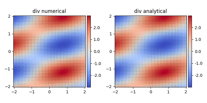
---------- 更新版本：包含差分步骤 ----------------

感谢@henry的评论，np.gradient默认步长为1，因此结果可能存在一些不匹配。我们可以提供自定义的差分步长。

#https://dev59.com/vGgu5IYBdhLWcg3wTFOi#47905007
import numpy as np
import matplotlib.pyplot as plt
from mpl_toolkits.axes_grid1 import make_axes_locatable

NY = 50
ymin = -2.
ymax = 2.
dy = (ymax -ymin )/(NY-1.)

NX = NY
xmin = -2.
xmax = 2.
dx = (xmax -xmin)/(NX-1.)


def divergence(f,h):
    """
    div(F) = dFx/dx + dFy/dy + ...
    g = np.gradient(Fx,dx, axis=1)+ np.gradient(Fy,dy, axis=0) #2D
    g = np.gradient(Fx,dx, axis=2)+ np.gradient(Fy,dy, axis=1) +np.gradient(Fz,dz,axis=0) #3D
    """
    num_dims = len(f)
    return np.ufunc.reduce(np.add, [np.gradient(f[i], h[i], axis=i) for i in range(num_dims)])

y = np.array([ ymin + float(i)*dy for i in range(NY)])
x = np.array([ xmin + float(i)*dx for i in range(NX)])

x, y = np.meshgrid( x, y, indexing = 'ij', sparse = False)

Fx  = np.cos(x + 2*y)
Fy  = np.sin(x - 2*y)

F = [Fx, Fy]
h = [dx, dy]



print('plotting')
rows = 1
cols = 2
#plt.clf()
plt.figure(figsize=(cols*3.5,rows*3.5))
plt.minorticks_on()


#g = np.gradient(Fx,dx, axis=1)+np.gradient(Fy,dy, axis=0) # equivalent to our func
g = divergence(F,h)
ax = plt.subplot(rows,cols,1,aspect='equal',title='div numerical')
#im=plt.pcolormesh(x, y, g)
im = plt.pcolormesh(x, y, g, shading='nearest', cmap=plt.cm.get_cmap('coolwarm'))
plt.quiver(x,y,Fx,Fy)
divider = make_axes_locatable(ax)
cax = divider.append_axes("right", size="5%", pad=0.05)
cbar = plt.colorbar(im, cax = cax,format='%.1f')


g = -np.sin(x+2*y) -2*np.cos(x-2*y)
ax = plt.subplot(rows,cols,2,aspect='equal',title='div analytical')
im=plt.pcolormesh(x, y, g)
im = plt.pcolormesh(x, y, g, shading='nearest', cmap=plt.cm.get_cmap('coolwarm'))
plt.quiver(x,y,Fx,Fy)
divider = make_axes_locatable(ax)
cax = divider.append_axes("right", size="5%", pad=0.05)
cbar = plt.colorbar(im, cax = cax,format='%.1f')


plt.tight_layout()
plt.savefig( 'divergence.png', format = 'png')
plt.show()

- John Paul Qiang Chen

---

看一下你的colorbar中的最大数值，它是0.2，但应该是3！https://stackoverflow.com/questions/67970477/compute-divergence-with-python/67971515#67971515 - henry

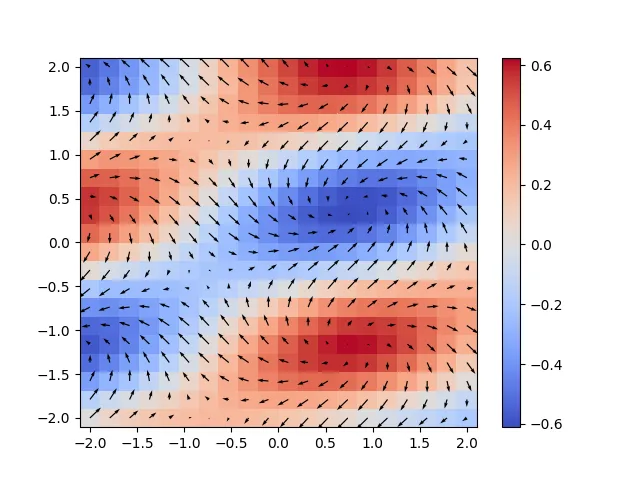
@henry 你说得对。事实上，numpy.gradient 的色条范围比解析结果略小。我周围的人通常不关心颜色范围。如果有人能解释一下为什么，我会很高兴的。@_@ - John Paul Qiang Chen

这是因为 no.gradient 使用的默认步长（1）与您的步长不对应。请参见此处：https://stackoverflow.com/questions/67970477/compute-divergence-with-python/67971515#67971515 - henry

奇怪的行为与增加分辨率的np.gradient。 - henry

这篇文章有一个拼写错误和一个逗号缺失，但是无法进行编辑。np.gradient(f) = df/dx, df/dy, df/dz[,] <+>... - Atcold

Answer 6

在@paul_chen的回答基础上，针对Matplotlib 3.3.0进行了一些补充（需要传递一个阴影参数，我猜默认的颜色映射已经改变了）

import numpy as np
import matplotlib.pyplot as plt

NY = 20; ymin = -2.; ymax = 2.
dy = (ymax -ymin )/(NY-1.)
NX = NY
xmin = -2.; xmax = 2.
dx = (xmax -xmin)/(NX-1.)

def divergence(f):
    num_dims = len(f)
    return np.ufunc.reduce(np.add, [np.gradient(f[i], axis=i) for i in range(num_dims)])

y = np.array([ ymin + float(i)*dy for i in range(NY)])
x = np.array([ xmin + float(i)*dx for i in range(NX)])

x, y = np.meshgrid( x, y, indexing = 'ij', sparse = False)

Fx  = np.cos(x + 2*y)
Fy  = np.sin(x - 2*y)


F = [Fx, Fy]
g = divergence(F)

plt.pcolormesh(x, y, g, shading='nearest', cmap=plt.cm.get_cmap('coolwarm'))
plt.colorbar()
plt.quiver(x,y,Fx,Fy)
plt.savefig( 'Div.png', format = 'png')

- BBSysDyn

---

这不完全正确！np. gradient 假定步长为 1，但这里步长是不同的。这就是为什么你得到的最大值大约是 0.6 而不是 3。参见：https://stackoverflow.com/questions/67970477/compute-divergence-with-python/67971515#67971515 - henry

Answer 7

据我所知，numpy中没有本地的发散函数。因此，计算发散的最佳方法是对梯度向量的分量求和，即计算发散。

- Joshua Cook

Answer 8

在Matlab中，差分作为内置函数被包含在其中，但在NumPy中却没有。这是一种或许值得投入到pylab中的东西，pylab是一个致力于创建可行的开源替代Matlab的努力。

http://wiki.scipy.org/PyLab

编辑：现在称为http://www.scipy.org/stackspec.html。

- Joshua Cook

Answer 9

之前计算散度的尝试都出现了错误！让我来给你展示一下：

我们有以下向量场 F：

F(x) = cos(x+2y)
F(y) = sin(x-2y)

如果我们使用Mathematica计算散度：

Div[{Cos[x + 2*y], Sin[x - 2*y]}, {x, y}]

我们得到：

-2 Cos[x - 2 y] - Sin[x + 2 y]

在 y [-1,2] 和 x [-2,2] 范围内具有最大值的：

N[Max[Table[-2 Cos[x - 2 y] - Sin[x + 2 y], {x, -2, 2 }, {y, -2, 2}]]] = 2.938

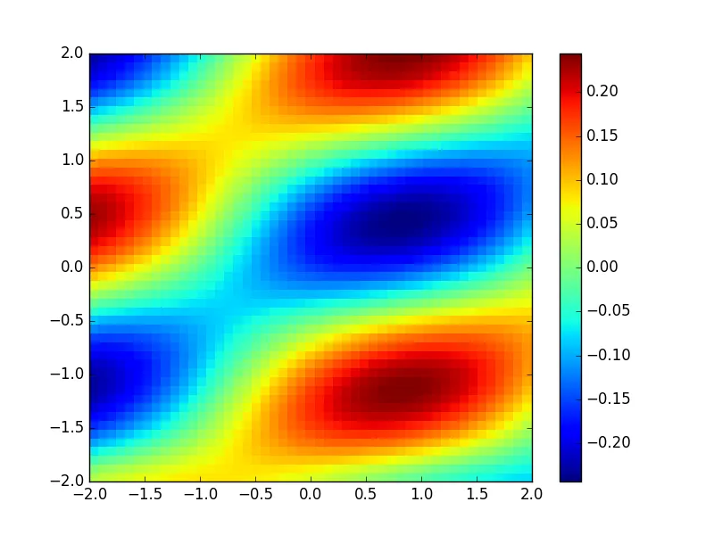
使用此处给出的散度方程：

def divergence(f):
        num_dims = len(f)
        return np.ufunc.reduce(np.add, [np.gradient(f[i], axis=i) for i in range(num_dims)])

我们得到了一个最大值约为0.625

正确的散度函数: Python计算散度

- henry

Answer 10

我认为@Daniel的答案不正确，特别是当输入按顺序排列时[Fx, Fy, Fz, ...]。

一个简单的测试用例

请参阅MATLAB代码：

a = [1 2 3;1 2 3; 1 2 3];
b = [[7 8 9] ;[1 5 8] ;[2 4 7]];
divergence(a,b)

这将给出结果：

ans =

   -5.0000   -2.0000         0
   -1.5000   -1.0000         0
    2.0000         0         0

丹尼尔的解决方案：

def divergence(f):
    """
    Daniel's solution
    Computes the divergence of the vector field f, corresponding to dFx/dx + dFy/dy + ...
    :param f: List of ndarrays, where every item of the list is one dimension of the vector field
    :return: Single ndarray of the same shape as each of the items in f, which corresponds to a scalar field
    """
    num_dims = len(f)
    return np.ufunc.reduce(np.add, [np.gradient(f[i], axis=i) for i in range(num_dims)])


if __name__ == '__main__':
    a = np.array([[1, 2, 3]] * 3)
    b = np.array([[7, 8, 9], [1, 5, 8], [2, 4, 7]])
    div = divergence([a, b])
    print(div)
    pass

这将会提供：

[[1.  1.  1. ]
 [4.  3.5 3. ]
 [2.  2.5 3. ]]

解释

Daniel的解决方案的错误在于，在Numpy中，x轴是最后一个轴而不是第一个轴。当使用np.gradient(x, axis=0)时，Numpy实际上给出了y方向的梯度（当x是一个二维数组时）。

我的解决方案

这是基于Daniel的答案的我的解决方案。

def divergence(f):
    """
    Computes the divergence of the vector field f, corresponding to dFx/dx + dFy/dy + ...
    :param f: List of ndarrays, where every item of the list is one dimension of the vector field
    :return: Single ndarray of the same shape as each of the items in f, which corresponds to a scalar field
    """
    num_dims = len(f)
    return np.ufunc.reduce(np.add, [np.gradient(f[num_dims - i - 1], axis=i) for i in range(num_dims)])

在我的测试案例中，它提供了与MATLAB divergence 相同的结果。

- huangbiubiu

---

在笛卡尔索引约定中，MATLAB用于meshgrid的是笛卡尔索引，NumPy用于meshgrid的是“xy”索引。因此，x轴只是第二个轴（x和y被交换）。因此，丹尼尔的解决方案将适用于[Fy，Fx，Fz，...]，其中所有Fn都是笛卡尔索引。您的“解决方案”颠倒了一切的顺序，并且对于维度> 2不会按预期工作，因为它适用于[...，Fz'，Fy'，Fx']，其中每个Fn'的轴的顺序相反。对于矩阵索引，丹尼尔的解决方案可以直接使用。 - Jonathan Jeffrey