计算和绘制矢量场

Question

我正尝试使用以下公式为给定的物体绘制一个势场：

U=-α_goal*e^(-((x-x_goal )^2/a_goal +(y-y_goal^2)/b_goal ) )

使用以下代码

    # Set limits and number of points in grid
    xmax = 10.0
    xmin = -xmax
    NX = 20
    ymax = 10.0
    ymin = -ymax
    NY = 20
    # Make grid and calculate vector components
    x = linspace(xmin, xmax, NX)
    y = linspace(ymin, ymax, NY)
    X, Y = meshgrid(x, y)
    x_obstacle = 0
    y_obstacle = 0
    alpha_obstacle = 1
    a_obstacle = 1
    b_obstacle = 1
    P = -alpha_obstacle * exp(-(X - x_obstacle)**2 / a_obstacle + (Y - y_obstacle)**2 / b_obstacle)
    Ey,Ex = gradient(P)
    print Ey
    print Ex

    QP = quiver(X, Y, Ex, Ey)

    show()

这段代码计算了一个势场。如何漂亮地绘制这个势场？另外，对于给定的势场，将其转换为矢量场的最佳方法是什么？（矢量场是势场的负梯度。）

我会非常感谢任何帮助。

我尝试使用np.gradient()函数，但结果并不是我所期望的：

我期望的结果应该类似于：

编辑： 在代码的两行中进行更改后：

y, x = np.mgrid[500:-100:200j, 1000:-100:200j] 
p = -1 * np.exp(-((x - 893.6)**2 / 1000 + (y - 417.35)**2 / 1000))

我的绘图有问题：左右翻转了（箭头位置正确但不是场的位置）： 编辑： 通过更改 y, x = np.mgrid[500:-100:200j, -100:1000:200j]进行修复。有什么想法吗？

- Tad

---

听起来你想要一个 matplotlib quiver plot。 - Cory Kramer

是的，我已经查看了quiver函数。鉴于我的P公式，如何从http://matplotlib.org/api/pyplot_api.html#matplotlib.pyplot.quiver获取U和V？我认为我的公式只是给出每个位置的势能值而不是向量。我有什么遗漏吗？ - Tad

@Tad - 使用 numpy.gradient 获取势场的梯度。例如，在你上面的例子中，使用 v, u = np.gradient(P)。它返回 dy，dx 而不是 dx，dy，因为 NumPy 数组是按行、列索引而不是按列、行索引。 - Joe Kington

谢谢Joe，我确实尝试了那种方法 - 我已经更新了我的帖子以展示我得到的结果。你能告诉我我做错了什么吗？ - Tad

Answer 1

首先，让我们在常规网格上对其进行评估，类似于您的示例代码。（顺便提一句，您的方程求值代码中有一个错误。它缺少exp内部的负号。）：

import numpy as np
import matplotlib.pyplot as plt

# Set limits and number of points in grid
y, x = np.mgrid[10:-10:100j, 10:-10:100j]

x_obstacle, y_obstacle = 0.0, 0.0
alpha_obstacle, a_obstacle, b_obstacle = 1.0, 1e3, 2e3

p = -alpha_obstacle * np.exp(-((x - x_obstacle)**2 / a_obstacle
                               + (y - y_obstacle)**2 / b_obstacle))

接下来，我们需要计算梯度（这是一种简单的有限差分方法，与上述函数的解析导数计算不同）：

# For the absolute values of "dx" and "dy" to mean anything, we'll need to
# specify the "cellsize" of our grid.  For purely visual purposes, though,
# we could get away with just "dy, dx = np.gradient(p)".
dy, dx = np.gradient(p, np.diff(y[:2, 0]), np.diff(x[0, :2]))

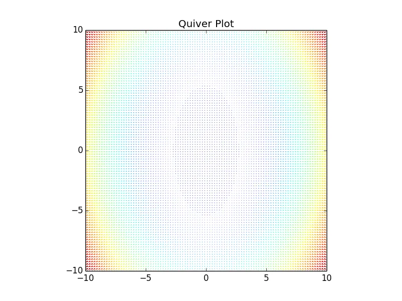
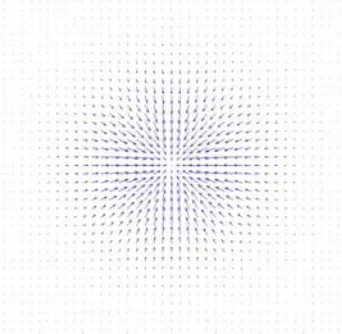
现在我们可以制作“箭头图”，但是结果可能不会像您期望的那样，因为在网格上的每个点都显示了一个箭头：

fig, ax = plt.subplots()
ax.quiver(x, y, dx, dy, p)
ax.set(aspect=1, title='Quiver Plot')
plt.show()

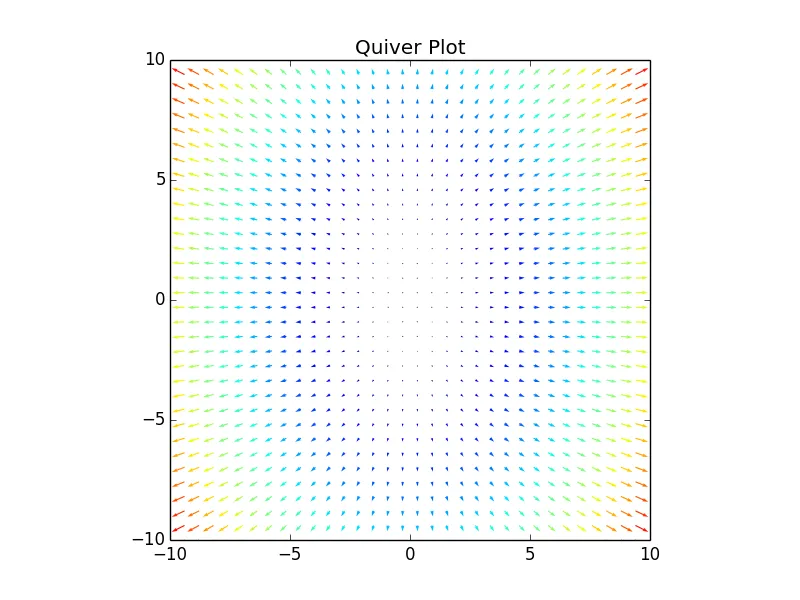
让箭头变大。最简单的方法是绘制每n个箭头，并让matplotlib处理自动缩放。我们在此处使用每3个点。如果您想要更少但更大的箭头，请将3更改为较大的整数。

# Every 3rd point in each direction.
skip = (slice(None, None, 3), slice(None, None, 3))

fig, ax = plt.subplots()
ax.quiver(x[skip], y[skip], dx[skip], dy[skip], p[skip])
ax.set(aspect=1, title='Quiver Plot')
plt.show()

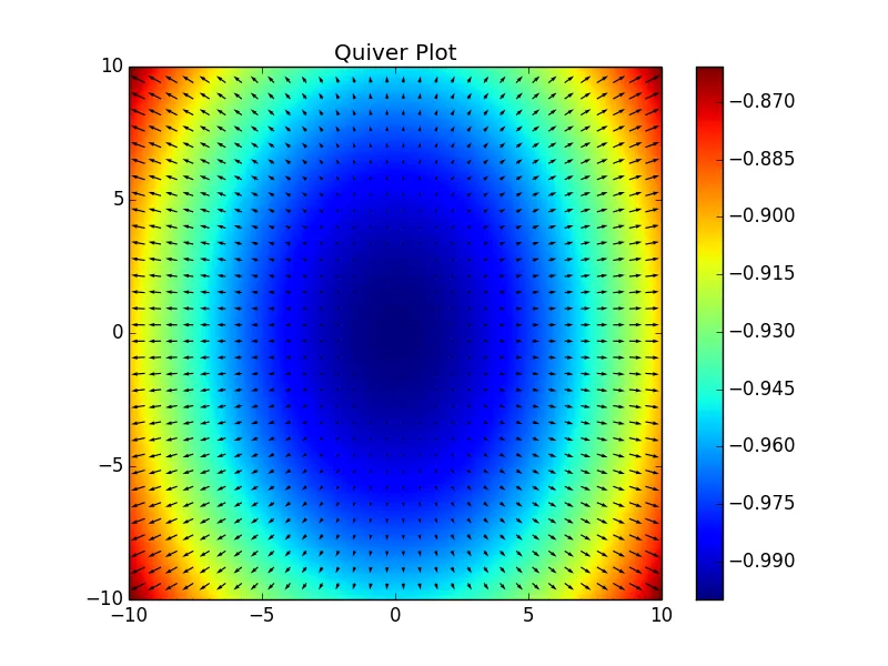
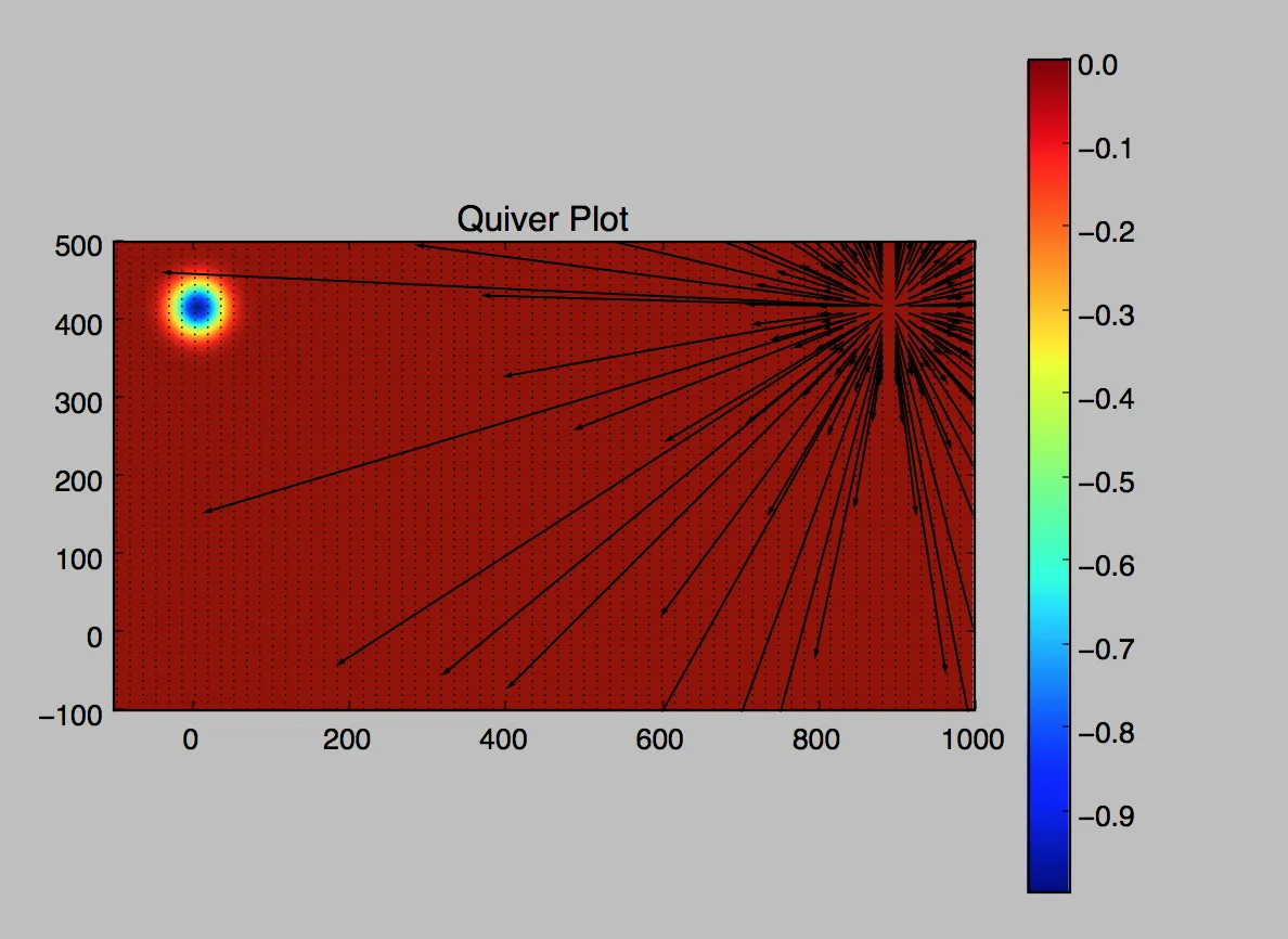
还不错，但是那些箭头仍然很难看到。更好的可视化方法可能是使用带有黑色渐变箭头覆盖的图像绘制：

skip = (slice(None, None, 3), slice(None, None, 3))

fig, ax = plt.subplots()
im = ax.imshow(p, extent=[x.min(), x.max(), y.min(), y.max()])
ax.quiver(x[skip], y[skip], dx[skip], dy[skip])

fig.colorbar(im)
ax.set(aspect=1, title='Quiver Plot')
plt.show()

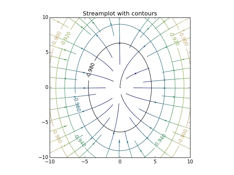
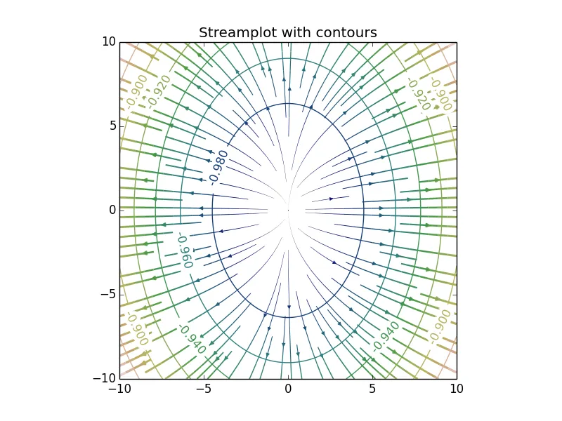
理想情况下，我们希望使用不同的色图或更改箭头颜色。 我会把那部分留给你。 你也可以考虑使用等值线图（ax.contour(x, y, p)）或流线图(ax.streamplot(x, y, dx, dy)来展示一个快速的例子:

fig, ax = plt.subplots()

ax.streamplot(x, y, dx, dy, color=p, density=0.5, cmap='gist_earth')

cont = ax.contour(x, y, p, cmap='gist_earth')
ax.clabel(cont)

ax.set(aspect=1, title='Streamplot with contours')
plt.show()

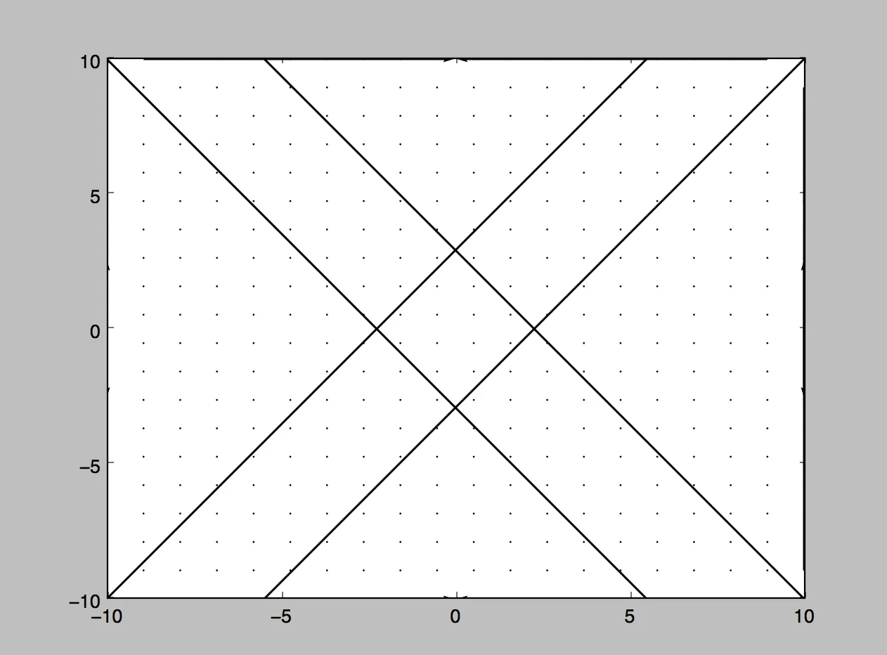
...为了变得更加花哨而言：

from matplotlib.patheffects import withStroke

fig, ax = plt.subplots()

ax.streamplot(x, y, dx, dy, linewidth=500*np.hypot(dx, dy),
              color=p, density=1.2, cmap='gist_earth')

cont = ax.contour(x, y, p, cmap='gist_earth', vmin=p.min(), vmax=p.max())
labels = ax.clabel(cont)

plt.setp(labels, path_effects=[withStroke(linewidth=8, foreground='w')])

ax.set(aspect=1, title='Streamplot with contours')
plt.show()

- Joe Kington

---

哇，这太棒了！我会仔细看你的代码，但现在想要感谢你的出色回复！ - Tad

很高兴能为您提供帮助！如果有任何不清楚的地方或遇到任何问题，随时都可以问我。 - Joe Kington

小心使用 numpy.gradient -- 默认步长为1，因此在上面的示例中结果不会被正确缩放。 - pv.

@pv - 很好的观点！在这种情况下，它不会产生任何视觉效果，但是你指出的dx和dy的绝对值完全错误。已更新答案以使用步长。谢谢！ - Joe Kington

@JoeKington，你知道我如何在上面绘制一个矢量位势场吗？即，在我进行绘制场的箭头之后，我想以一种不会破坏自动缩放的方式添加几个矢量。谢谢！ - Tad