numpy.polyfit的错误是什么？

Question

我想使用 numpy.polyfit 进行物理计算，因此我需要误差的数量级。

- varantir

Answer 1

如果在调用polyfit时指定full=True，它将包括额外的信息：

>>> x = np.arange(100)
>>> y = x**2 + 3*x + 5 + np.random.rand(100)
>>> np.polyfit(x, y, 2)
array([ 0.99995888,  3.00221219,  5.56776641])
>>> np.polyfit(x, y, 2, full=True)
(array([ 0.99995888,  3.00221219,  5.56776641]), # coefficients
 array([ 7.19260721]), # residuals
 3, # rank
 array([ 11.87708199,   3.5299267 ,   0.52876389]), # singular values
 2.2204460492503131e-14) # conditioning threshold

返回的残差值是拟合误差平方和，不确定这是否符合您的要求：

>>> np.sum((np.polyval(np.polyfit(x, y, 2), x) - y)**2)
7.1926072073491056

在版本1.7中还有一个关键字，它将返回您的系数的协方差矩阵，您可以使用它来计算拟合系数本身的不确定性。

- Jaime

---

你知道 np.polyfit 在寻找最佳拟合时是否使用 TLS（全局最小二乘法，也称为正交最小二乘法）或 OLS（普通最小二乘法）吗？ - Oliver Angelil

np.polyfit 使用普通最小二乘算法，使用 np.linalg.lstsq，类似于 scipy.linalg.lstsq。scipy.odr 实现正交最小二乘算法，更精确地说是正交距离回归。 - Cibin Joseph

Answer 2

正如您在文档中所看到的：

Returns
-------
p : ndarray, shape (M,) or (M, K)
    Polynomial coefficients, highest power first.
    If `y` was 2-D, the coefficients for `k`-th data set are in ``p[:,k]``.

residuals, rank, singular_values, rcond : present only if `full` = True
    Residuals of the least-squares fit, the effective rank of the scaled
    Vandermonde coefficient matrix, its singular values, and the specified
    value of `rcond`. For more details, see `linalg.lstsq`.

这意味着如果您进行拟合并得到残差如下：

 import numpy as np
 x = np.arange(10)
 y = x**2 -3*x + np.random.random(10)

 p, res, _, _, _ = numpy.polyfit(x, y, deg, full=True)

然后，p 是您的拟合参数，res 将是残差，就像上面描述的那样。下划线是因为您不需要保存最后三个参数，所以可以将它们保存在变量 _ 中，您不会使用它们。这是一种惯例，不是必需的。

---

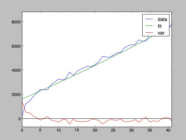
@Jaime 的回答解释了残差的含义。你可以看看那些平方偏差的函数（其总和为res）。这对于查看未充分拟合的趋势特别有帮助。残差可能很大是由于统计噪声，或者可能是由于系统的拟合较差造成的，例如：

x = np.arange(100)
y = 1000*np.sqrt(x) + x**2 - 10*x + 500*np.random.random(100) - 250

p = np.polyfit(x,y,2) # insufficient degree to include sqrt

yfit = np.polyval(p,x)

figure()
plot(x,y, label='data')
plot(x,yfit, label='fit')
plot(x,yfit-y, label='var')

因此在这张图中，请注意 x=0 附近的拟合不好:

- askewchan