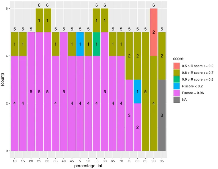
我想在堆积条形图的顶部添加一个总计数,除了我已有的不同类别的计数之外。
这是我的图表:
所以在10(x轴上的第一个)处,我将有5,然后又是5等等。
我找到了很多关于这个问题的帖子,但没有一个能让我解决我的问题。我可能最接近的是这个帖子:如何在stat_summary ggplot中添加观测计数标签?但问题是我需要获取"因子"的字符串计数。
这是上面图表的代码:
ggplot(my_df, aes(x=percentage_int, fill = score)) +
  geom_bar(aes(y = (..count..))) +
  geom_text(stat='count', aes(label=..count..),position = position_stack(vjust = 0.5))
这是我从上面的文章中改编的代码:
label_df = my_df %>% group_by(percentage_int) %>% summarise(n=n())

ggplot(my_df, aes(x=percentage_int, fill = score)) +
          geom_bar(aes(y = (..count..))) +
          geom_text(stat='count', aes(label=..count..),position = position_stack(vjust = 0.5)) +
          geom_text(data=label_df,aes(fill = score, x = percentage_int, label=n))
我不太确定为什么它不起作用...
看来我无法避免为此创建额外的 df...
如果有 stat_summary 的解决方案也很好,因为我也尝试过。谢谢!
以下是我的数据测试:
structure(list(percentage_int = structure(c(13L, 17L, 10L, 9L,
14L, 8L, 19L, 11L, 18L, 12L, 6L, 15L, 4L, 16L, 5L, 2L, 20L, 3L,
7L, 13L, 17L, 18L, 12L, 4L, 11L, 3L, 14L, 2L, 19L, 15L, 7L, 16L,
6L, 8L, 5L, 20L, 10L, 9L, 19L, 8L, 9L, 11L, 12L, 20L, 13L, 14L,
10L, 18L, 15L, 16L, 3L, 5L, 17L, 4L, 2L, 7L, 6L, 17L, 5L, 19L,
7L, 18L, 9L, 20L, 14L, 16L, 11L, 8L, 3L, 13L, 10L, 6L, 4L, 15L,
12L, 2L, 16L, 18L, 19L, 14L, 13L, 20L, 7L, 17L, 15L, 2L, 9L,
5L, 3L, 4L, 12L, 10L, 6L, 11L, 8L, 6L, 19L, 13L, 5L, 12L), .Label = c("0",
"10", "15", "20", "25", "30", "35", "40", "45", "5", "50", "55",
"60", "65", "70", "75", "80", "85", "90", "95"), class = "factor"),
    score = c("Rscore = 0.96", "Rscore = 0.96", "Rscore = 0.96",
    "Rscore = 0.96", "Rscore = 0.96", "Rscore = 0.96", "0.8 > R score >= 0.7",
    "Rscore = 0.96", "0.8 > R score >= 0.7", "Rscore = 0.96",
    "Rscore = 0.96", "Rscore = 0.96", "Rscore = 0.96", "Rscore = 0.96",
    "Rscore = 0.96", "Rscore = 0.96", "0.8 > R score >= 0.7",
    "Rscore = 0.96", "Rscore = 0.96", "Rscore = 0.96", "Rscore = 0.96",
    "0.8 > R score >= 0.7", "Rscore = 0.96", "Rscore = 0.96",
    "Rscore = 0.96", "Rscore = 0.96", "Rscore = 0.96", "Rscore = 0.96",
    "0.5 > R score >= 0.2", "Rscore = 0.96", "Rscore = 0.96",
    "Rscore = 0.96", "Rscore = 0.96", "Rscore = 0.96", "Rscore = 0.96",
    "0.8 > R score >= 0.7", "Rscore = 0.96", "Rscore = 0.96",
    "0.8 > R score >= 0.7", "Rscore = 0.96", "0.8 > R score >= 0.7",
    "0.8 > R score >= 0.7", "0.8 > R score >= 0.7", NA, "0.8 > R score >= 0.7",
    "0.8 > R score >= 0.7", "R score < 0.2", "0.8 > R score >= 0.7",
    "Rscore = 0.96", "Rscore = 0.96", "0.8 > R score >= 0.7",
    "0.8 > R score >= 0.7", "R score < 0.2", "Rscore = 0.96",
    "0.8 > R score >= 0.7", "0.8 > R score >= 0.7", "0.8 > R score >= 0.7",
    "0.8 > R score >= 0.7", "Rscore = 0.96", "0.8 > R score >= 0.7",
    "Rscore = 0.96", "0.8 > R score >= 0.7", "Rscore = 0.96",
    NA, "Rscore = 0.96", "0.8 > R score >= 0.7", "Rscore = 0.96",
    "Rscore = 0.96", "Rscore = 0.96", "Rscore = 0.96", "Rscore = 0.96",
    "Rscore = 0.96", "Rscore = 0.96", "0.8 > R score >= 0.7",
    "Rscore = 0.96", "Rscore = 0.96", "0.8 > R score >= 0.7",
    "0.8 > R score >= 0.7", "0.8 > R score >= 0.7", "Rscore = 0.96",
    "Rscore = 0.96", NA, "Rscore = 0.96", "0.8 > R score >= 0.7",
    "Rscore = 0.96", "Rscore = 0.96", "Rscore = 0.96", "Rscore = 0.96",
    "Rscore = 0.96", "Rscore = 0.96", "Rscore = 0.96", "Rscore = 0.96",
    "Rscore = 0.96", "Rscore = 0.96", "Rscore = 0.96", "Rscore = 0.96",
    "0.5 > R score >= 0.2", "Rscore = 0.96", "Rscore = 0.96",
    "0.9 > R score >= 0.8")), row.names = c("1410", "1411", "1412",
"1413", "1414", "1415", "1416", "1417", "1418", "1419", "1420",
"1421", "1422", "1423", "1424", "1425", "1426", "1427", "1428",
"1448", "1449", "1450", "1451", "1452", "1453", "1454", "1455",
"1456", "1457", "1458", "1459", "1460", "1461", "1462", "1463",
"1464", "1465", "1466", "1619", "1620", "1621", "1622", "1623",
"1624", "1625", "1626", "1627", "1628", "1629", "1630", "1631",
"1632", "1633", "1634", "1635", "1636", "1637", "1771", "1772",
"1773", "1774", "1775", "1776", "1777", "1778", "1779", "1780",
"1781", "1782", "1783", "1784", "1785", "1786", "1787", "1788",
"1789", "1828", "1829", "1830", "1831", "1832", "1833", "1834",
"1835", "1836", "1837", "1838", "1839", "1840", "1841", "1842",
"1843", "1844", "1845", "1846", "1885", "1886", "1887", "1888",
"1889"), class = "data.frame")